Mapping Sensitivity in Jaw-Shape Evolutionary Rates with rateMap, Part 1

Overview

The jaw-shape vignette fits one conservative bifrost search to Paleozoic fish lower-jaw shape data from Troyer et al. (2025). It then colors the selected SIMMAP-style tree by fitted regime-specific rates.

Here we use rateMap() in two steps. First, compute a reusable "rateMap" object from a list of completed bifrost searches. Then, call plot() on that object to render a first-pass equal-weight map, inspect the fitted-rate range, and redraw the map with explicit near-zero metadata. Because ordinary bifrost shifts occur at nodes, the default computed summary is one fitted log-rate per branch.

The same rate-diagnostic controls can be used with a single fitted search; here we introduce them after the first-pass sensitivity map, where the broad fitted-rate range makes the display choice visible.

Methodologically, rateMap() follows the phytools SIMMAP plotting ecosystem: it is a rate-valued analogue of densityMap(), and the plot method renders through plotSimmap() and plotTree(). Details and acknowledgements are collected near the end of the vignette and in ?plot.rateMap.

This vignette is self-contained for the rateMap() workflow, while the biological setup comes from the main jaw-shape analysis. Long-running search chunks are shown for interactive use; run them once, save the fitted objects, and then use the lighter rateMap() chunks for summaries and plot(x, ...) chunks for display. Part 2 continues with IC weighting, uncertainty views, and same-topology tree samples.

Figure 1. Single-run branch-rate visualization from the jaw-shape example. This tree shows the fitted branch-rate categories for one selected bifrost search on the jaw-shape data; branch colors encode the regime-specific fitted evolutionary rates from that single model. The multi-run rateMap() workflow below asks which parts of this single-run pattern persist when the search threshold changes; subsequent maps use log fitted rates by default.

Why a Threshold Sweep?

Simulation-based assessment is the primary way to evaluate method-level performance because the generating model, true shift locations, and true rates are known. Simulations ask whether a threshold recovers real shifts, avoids false positives, and behaves well across tree sizes, trait dimensions, and effect sizes. The GIC threshold used in the main jaw-shape analysis follows that logic: values near 20 are conservative, but neighboring thresholds still deserve a dataset-specific sensitivity check.

The sweep here asks a narrower empirical question: does the jaw-shape rate pattern persist as the shift acceptance threshold becomes more or less conservative? rateMap() turns repeated bifrost searches into branchwise summaries that help distinguish high-rate regions that persist across threshold settings from features that appear only under permissive settings. This complements simulation-based model-performance assessment: simulations benchmark the method, while threshold sweeps diagnose robustness in this dataset.

We keep min_descendant_tips fixed throughout the sweep. That argument defines which internal nodes may receive candidate shifts; changing it would change the candidate-shift universe and the evidence threshold at the same time. Holding it constant isolates the acceptance threshold. For the jaw-shape data, min_descendant_tips = 10 also avoids fitting separate high-dimensional covariance structure to very small clades. That value is a worked-example choice, not a general default: real analyses may need smaller or larger values depending on tree size, trait dimensionality, and the smallest clades that should be allowed to carry their own fitted regime.

Setup

Load the packages used in the jaw-shape workflow. geomorph::two.d.array() converts the packaged landmark array into a two-dimensional species-by-trait matrix, matching the setup in the main jaw-shape vignette.

library(bifrost)
library(ape)
library(phytools)
library(geomorph)

Load and align the same data used in the jaw-shape vignette.

tree_path <- system.file(
  "extdata", "jaw-shape", "mrbayes_prune_tree.RDS",
  package = "bifrost"
)
landmark_path <- system.file(
  "extdata", "jaw-shape", "jaws_coords.RDS",
  package = "bifrost"
)

fish.tree <- readRDS(tree_path)
landmarks <- readRDS(landmark_path)

fish.tree <- ladderize(untangle(as.phylo(fish.tree)))
fish.data <- two.d.array(landmarks)
fish.data <- fish.data[match(fish.tree$tip.label, rownames(fish.data)), ]

stopifnot(identical(rownames(fish.data), fish.tree$tip.label))

Run the Sensitivity Sweep

The main jaw-shape vignette uses shift_acceptance_threshold = 20. We include that value and several neighboring choices. Lower thresholds accept smaller IC improvements; higher thresholds usually accept fewer shifts.

threshold_grid <- c(10, 15, 20, 25, 30, 40)
min_tips <- 10

Use a helper function so every run differs only in the IC threshold. Per-shift support weights from searchOptimalConfiguration() are optional here: set uncertaintyweights_par = TRUE only if you need those diagnostics for each individual search. They differ from the fit-level weights used by rateMap(weights = "ic"), which come from each retained run’s optimal_ic and IC_used.

Think of rateMap() as the post-processing compute step: it extracts fitted branch-rate trees and regime-rate parameters, matches branches across retained runs, and returns a reusable "rateMap" object. The common compute controls in this vignette are weights, uncertainty, summary, and log. Once the object exists, use plot(x, ...) for display. Most users can stop there. Use rateMapView(x, ...) only when you want to freeze a display mapping before printing category tables or reusing the exact same categories in multiple figures. More specialized controls can be passed as control = list(...) or built with rateMapControl(); these are mainly for posterior-tree samples, interval maps, custom extractors, or large sensitivity sets.

The sweep is the slowest part of the workflow. The examples below save the fitted searches to a local cache and reload them for the lighter rateMap() summaries. Run the sweep chunk once, then reuse the saved results while exploring display, weighting, and uncertainty options.

run_jaw_threshold <- function(threshold) {
  searchOptimalConfiguration(
    baseline_tree              = fish.tree,
    trait_data                 = fish.data,
    formula                    = "trait_data ~ 1",
    min_descendant_tips        = min_tips,
    num_cores                  = 4,
    shift_acceptance_threshold = threshold,
    uncertaintyweights_par     = FALSE,
    IC                         = "GIC",
    method                     = "H&L",
    error                      = TRUE,
    plot                       = FALSE,
    store_model_fit_history    = FALSE,
    verbose                    = TRUE
  )
}

set.seed(1)
jaw_threshold_runs <- lapply(threshold_grid, run_jaw_threshold)
names(jaw_threshold_runs) <- paste0("GIC_threshold_", threshold_grid)

cache_path <- rate_map_cache_path()
dir.create(dirname(cache_path), recursive = TRUE, showWarnings = FALSE)
saveRDS(jaw_threshold_runs, cache_path)

If the searches have already been run, load the saved results instead.

cache_path <- rate_map_cache_path()
if (!file.exists(cache_path)) {
  stop("No jaw-shape threshold cache found; run the sweep chunk first.")
}
jaw_threshold_runs <- readRDS(cache_path)
threshold_grid <- as.numeric(sub("GIC_threshold_", "", names(jaw_threshold_runs)))

Before mapping rates, inspect how the selected model changes across the sweep.

sweep_summary <- data.frame(
  threshold = threshold_grid,
  n_shifts = vapply(
    jaw_threshold_runs,
    function(x) length(x$shift_nodes_no_uncertainty),
    integer(1)
  ),
  baseline_ic = vapply(jaw_threshold_runs, `[[`, numeric(1), "baseline_ic"),
  optimal_ic = vapply(jaw_threshold_runs, `[[`, numeric(1), "optimal_ic"),
  IC_used = vapply(jaw_threshold_runs, `[[`, character(1), "IC_used")
)
sweep_summary$delta_ic <- sweep_summary$baseline_ic - sweep_summary$optimal_ic
sweep_summary

threshold	n_shifts	baseline_ic	optimal_ic	IC_used	delta_ic
10	19	-335266.3	-342617.0	GIC	7350.7
15	13	-335266.3	-342531.2	GIC	7264.9
20	17	-335266.3	-342739.4	GIC	7473.1
25	14	-335266.3	-342455.1	GIC	7188.8
30	15	-335266.3	-342733.4	GIC	7467.2
40	12	-335266.3	-342409.2	GIC	7142.9

Table 1. Observed threshold sweep. Each row is one completed search with min_descendant_tips = 10. threshold is the shift-acceptance threshold; n_shifts is the number of retained shifts; baseline_ic and optimal_ic compare the unshifted and selected models; IC_used records the criterion; and delta_ic is baseline_ic - optimal_ic. Accepted shifts are not perfectly monotonic because changing the threshold can alter the greedy search path, not just trim a fixed list of candidate shifts.

This table gives a first diagnostic. In this run, the main jaw-shape threshold (20) gives the lowest GIC among the six retained searches, closely followed by threshold 30. Those two model outcomes dominate the IC-weighted rate map in Part 2.

Equal-Weight Rate Map

A simple first diagnostic gives every threshold run equal weight. This asks whether the same branch log-rate pattern appears across the threshold settings considered here.

By default, rateMap() follows bifrost’s branch-level framing: shifts occur at nodes, so each branch receives one summarized fitted rate. With the default log = TRUE, across-run means are mean log-rates, equivalent to the log of a weighted geometric mean on the original rate scale.

plot(x, ...) then colors those branch summaries as ordered log-rate categories. In multi-run summaries, these categories are plotting bins for summarized branch values; they should not be read as newly inferred bifrost regimes. For branch summaries, rate_categories reports how many branches fall into each displayed bin and summarizes the plotted branch values assigned to that bin.

Branch maps also carry rate diagnostics for near-zero or isolated high-tail rates. These diagnostics add rate_flag metadata without removing branches or changing fitted values. By default, no near-zero rule is applied. Supplying zero_floor activates the manual floor rule; using method = "tail_cluster" requests the data-driven lower-tail diagnostic.

That conservative default matters because bifrost can infer very low but positive fitted rates for clades with little observed trait variation. Leaving those branches unflagged is not wrong; it shows the fitted branch summaries directly. If you have a biologically or numerically meaningful threshold in mind, supply zero_floor to mark rates below that value as effectively zero for display. rateMap() leaves that choice explicit rather than guessing a universal cutoff.

Start with the default map and inspect its range before deciding how to display it.

jaw_rate_map_equal_first <- rateMap(
  jaw_threshold_runs,
  weights = "equal",
  uncertainty = TRUE,
  progress = TRUE
)
jaw_rate_map_equal_first <- rateMapView(
  jaw_rate_map_equal_first,
  palette = "Viridis",
  legend_title = "Mean log fitted rate"
)

jaw_rate_map_equal_first
jaw_rate_map_equal_first$rate_diagnostics

#> rateMap object
#> - fits: 6
#> - summary: branch
#> - target: first
#> - check: full
#> - weights: equal
#> - uncertainty: TRUE
#> - color mode: category
#> - plotted value: value
#> - value range: -24.2 to -11.41
#> - rate flags: 0 near-zero, 0 high-outlier (method: none)
#> - fold range: 361384 full, 361384 regular
#> - sd range: 0.05957 to 5.979

diagnostic	value
method	none
near-zero floor	none
regular branches	170
near-zero branches	0
high-outlier branches	0
minimum fitted log-rate	-24.2
minimum regular fitted log-rate	-24.2
maximum fitted log-rate	-11.41
full fold range	361384
regular fold range	361384

Table 2. First-pass equal-weight rate diagnostics. The default diagnostic pass leaves all branches in the regular category, but the fitted log-rate range is still enormous. This is a flag that the researcher should inspect the map and fitted-rate range before accepting the default color scale.

The first pass is a useful warning rather than a final display choice. The branch summaries run from about -24.2 to -11.4 on the log-rate scale, which corresponds to original fitted rates of about 3.08e-11 to 1.11e-5. A 361,000-fold range is possible under the fitted model, but it is biologically hard to interpret as ordinary rate variation. That is the reason to inspect the lower tail and, when appropriate, display the effectively zero-rate branches as a separate diagnostic category. The default plot legend spans the prettier category boundaries, here -26 to -10, so its lower limit is a bin edge rather than the observed minimum branch summary.

plot(
  jaw_rate_map_equal_first,
  type = "arc",
  show_tip_labels = FALSE,
  legend_fsize = 0.9,
  arc_height = 0.5
)

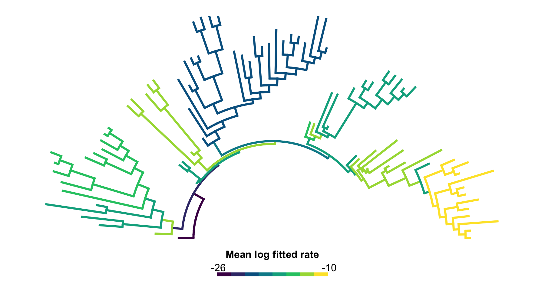
Figure 2. Default equal-weight branch-category rate map. This first-pass arc tree shows the unmodified default display: all branches are binned into the ordinary ordered log-rate categories, with no manual near-zero flagging.

In this jaw-shape example, the lowest-rate branches form a broader lower-tail cluster that deserves an explicit diagnostic display choice.

The second pass keeps the same fitted values but uses the tail_cluster diagnostic. This Otsu-style rule, adapted from Otsu’s histogram thresholding criterion (Otsu 1979), works on log-rates, chooses the guarded two-class split that maximizes separation between the tail and the remaining branches, and only accepts it when the lower cluster is separated from the regular branches and greatly reduces the regular fold range.

jaw_rate_map_equal <- rateMap(
  jaw_threshold_runs,
  weights = "equal",
  uncertainty = TRUE,
  progress = TRUE,
  control = rateMapControl(
    rate_flags = rateMapRateFlags(method = "tail_cluster")
  )
)
jaw_rate_map_equal <- rateMapView(
  jaw_rate_map_equal,
  palette = "Viridis",
  legend_title = "Mean log fitted rate"
)

jaw_rate_map_equal
jaw_rate_map_equal$rate_categories

After flagging, the grey near-zero category sits outside the ordered palette. The Viridis colors are regenerated for the remaining regular categories, so the unflagged branches use the full low-to-high color range. The legend still spans the full plotted data range and marks the cluster cutoff, here about -18.39, between the highest near-zero branch (-19.79) and the first regular branch (-16.99). In this example the first occupied regular automatic bin starts at -17; use explicit category_breaks if you want the display anchored to a particular numeric cutoff.

#> rateMap object
#> - fits: 6
#> - summary: branch
#> - target: first
#> - check: full
#> - weights: equal
#> - uncertainty: TRUE
#> - color mode: category
#> - plotted value: value
#> - value range: -24.2 to -11.41
#> - rate flags: 54 near-zero, 0 high-outlier (method: tail_cluster)
#> - fold range: 361384 full, 265 regular
#> - sd range: 0.05957 to 5.979

The category table and diagnostic table should be read together: the left table shows how branch summaries are binned for display, and the right table records the near-zero rule that created the grey category.

Table 3. Equal-weight rate categories after near-zero flagging. Ordered log-rate bins used to color the equal-weight branch-category map. rate_category is the displayed interval or special near-zero category; n_branches counts branches in each displayed category; and value_mean summarizes the plotted branch log-rates assigned to each bin.

rate_category	n_branches	value_mean
near-zero	54	-21.51
-17 to -16	40	-16.38
-16 to -15	4	-15.1
-15 to -14	18	-14.96
-14 to -13	16	-13.4
-13 to -12	16	-12.37
-12 to -11	22	-11.41

Table 4. Equal-weight rate diagnostics after near-zero flagging. Diagnostic companion to Table 3. method = "tail_cluster" marks the separated lower log-rate cluster as a display category without removing branches or changing fitted values. Fitted-rate bounds are shown on the plotted log scale.

diagnostic	value
method	tail_cluster
tail-cluster log cutoff	-18.39
tail-cluster log gap	2.803
tail-cluster fold reduction	1364
tail-cluster branch fraction	0.3176
regular branches	116
near-zero branches	54
high-outlier branches	0
minimum fitted log-rate	-24.2
minimum regular fitted log-rate	-16.99
maximum fitted log-rate	-11.41
full fold range	361384
regular fold range	265

The near-zero category is metadata, not a data filter. The full fitted-rate range is still available in jaw_rate_map_equal$intervals, but the ordinary rate bins and the visual color scale now describe the remaining regular branches rather than stretching across a numerical floor.

plot(
  jaw_rate_map_equal,
  type = "arc",
  show_tip_labels = FALSE,
  legend_fsize = 0.9,
  arc_height = 0.5
)

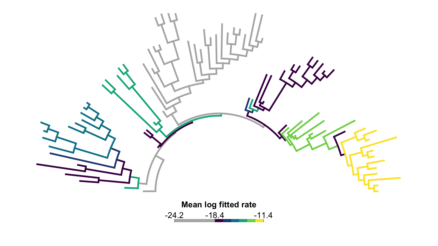
Figure 3. Equal-weight branch-category rate map after near-zero flagging. This arc tree summarizes the six GIC-threshold searches by giving each completed search the same weight. Branches in the separated lower log-rate cluster are shown as a separate grey category; remaining regular branches are colored by ordered categories of their mean fitted branch log-rate.

Each threshold run contributes one sixth of the branch log-rate summary. The highest mean log-rate region occurs in the lungfish-centered part of the tree, including branches descending toward Griphognathus, Holodipterus, Rhynchodipterus, and related taxa.

Interpret this map as a sensitivity average, not as a posterior probability map. Branches with consistently high log-rate values are repeatedly assigned to faster regimes across the threshold sweep; intermediate categories may reflect either genuinely moderate rates or a mixture of low- and high-rate assignments across thresholds.

If you want tighter control over the display categories after this diagnostic step, adjust the plotting bins directly.

plot(jaw_rate_map_equal, n_categories = 5)
plot(jaw_rate_map_equal, n_categories = 5, category_bin_method = "equal")
plot(jaw_rate_map_equal, category_breaks = c(-17, -15, -13, -11))

Practical Takeaways

• Holding min_descendant_tips = 10 fixed keeps the candidate-node filter constant while shift_acceptance_threshold changes.
• Equal weights summarize robustness across selected threshold settings.
• The first-pass rate diagnostics are part of the workflow: inspect the fitted-rate range before accepting the default color scale.
• The default diagnostic pass applies no near-zero rule; manual floors and broader tail structure should be requested explicitly.
• method = "tail_cluster" is display metadata, not a data filter. It uses an Otsu-style two-class split to mark a separated lower log-rate cluster while preserving fitted values in the output object.
• In plot(x, ...), n_categories sets the target number of automatic category bins; category_bin_method = "equal" and category_breaks give more direct bin control; ncolors controls continuous ramps.

Next Steps

Part 2 continues from this adjusted equal-weight map and asks how the interpretation changes under IC weighting, across-threshold uncertainty maps, same-topology tree samples, original-scale rates, and branch-level diagnostic tables.

Read Part 2: Weighting, uncertainty, and diagnostics.

Acknowledgements and Provenance

The core idea is adapted from phytools::densityMap(): summarize mapped histories on a shared tree and display the summary as a colored phylogeny. rateMap() changes the mapped quantity from posterior state probability to fitted branch-rate summaries from completed bifrost searches.

The drawing layer uses phytools::plotSimmap(), with phytools::plotTree() for outline and base-tree passes. plot.rateMap() forwards tree-layout controls such as type, fsize, ftype, lwd, mar, direction, offset, xlim, ylim, underscore, and arc_height; rate-map controls such as palette, color_mode, n_categories, category_breaks, legend_title, and near-zero diagnostics are handled by rateMap() before the colored tree is drawn.

This vignette was developed with assistance from OpenAI tools for drafting and editing; all scientific content, interpretation, and final decisions were reviewed by the authors.

References

• Clavel, J., Aristide, L., and Morlon, H. (2019). A Penalized Likelihood Framework for High-Dimensional Phylogenetic Comparative Methods and an Application to New-World Monkeys Brain Evolution. https://doi.org/10.1093/sysbio/syy045
• Otsu, N. (1979). A threshold selection method from gray-level histograms. IEEE Transactions on Systems, Man, and Cybernetics, 9(1), 62-66. https://doi.org/10.1109/TSMC.1979.4310076
• Paradis, E., and Schliep, K. (2019). ape 5.0: an environment for modern phylogenetics and evolutionary analyses in R. Bioinformatics, 35, 526-528. https://doi.org/10.1093/bioinformatics/bty633
• Revell, L. J. (2013). Two new graphical methods for mapping trait evolution on phylogenies. Methods in Ecology and Evolution, 4, 754-759.
• Revell, L. J. (2014). Graphical methods for visualizing comparative data on phylogenies. Chapter 4 in Modern Phylogenetic Comparative Methods and Their Application in Evolutionary Biology: Concepts and Practice, 77-103.
• Revell, L. J. (2024). phytools 2.0: an updated R ecosystem for phylogenetic comparative methods (and other things). PeerJ, 12, e16505. https://doi.org/10.7717/peerj.16505
• Troyer, E. M., et al. (2025). Macroevolutionary role reversals in the earliest radiation of bony fishes. https://doi.org/10.1016/j.cub.2025.08.008

Software Used in This Vignette

• bifrost for shift searches and rateMap() summaries.
• geomorph for converting landmark arrays to species-by-trait matrices.
• ape and phytools for phylogenetic data structures, SIMMAP trees, and plotting.