
Empirically Calibrated Simulations for bifrost, Part 1: Performance
Source:vignettes/simulation-study-part-1.Rmd
simulation-study-part-1.RmdDevelopment note: This simulation and tuning workflow is under active development and remains somewhat experimental. The interface and recommendations may change as it is evaluated more broadly.
This is Part 1 of the empirically calibrated simulation workflow. Here we examine performance at fixed search settings; Part 2 compares alternative settings on the same simulated datasets and shows how to pass selected settings to an empirical search.
How well does bifrost recover shifts in datasets
resembling your own? Here we assess performance using simulations
calibrated to the empirical tree, trait dimensionality, fitted means,
and residual covariance scale.
We then compare search behavior under three scenarios:
- a null model with no shifts, to estimate expected false positives,
- proportional covariance shifts, which match the fitted model, and
- an integration-rate scenario that departs from the fitted model, coupling reduced integration with faster marginal rates, or increased integration with slower marginal rates.
These simulations can guide search settings before an analysis or assess their performance afterward. Repeated subtree resampling lets us explore different topologies and parameter draws without searching the full tree in every replicate.
We use the passerine body-plan data from Berv et al. (2026) to calibrate this worked example. The simulations shown here are a new tutorial exercise, not the analyses reported in that study.
The saved summaries reproduce the tables below without fitting models or running simulations; the simulation examples are optional.
Start by loading bifrost.
This part requests the passerine tree (passerine-tree,
approximately 81 KB), trait matrix (passerine-traits,
approximately 212 KB), and simulation preview tables
(simulation-preview-tables, approximately 6 KB). First use
downloads and verifies each file; later calls reuse the verified cache.
The larger tree and trait files share that resolver cache with the
passerine articles. This explicit command checks for an updated preview
table:
# Refresh the preview tables only when an updated copy is wanted.
bifrost_example_file("simulation-preview-tables", refresh = TRUE)
Build an empirically calibrated template
Here we use the empirical calibration structure from Berv et al. (2026), which models 12 skeletal traits jointly while keeping log body mass as a phylogenetic covariate.
# Resolve the passerine tree and calibrated skeletal measurements.
tree_path <- bifrost_example_file("passerine-tree")
trait_path <- bifrost_example_file("passerine-traits")

# Align the trait rows to the tree's tip order.
bird_tree <- ape::read.tree(tree_path)
bodyplan_data <- readRDS(trait_path)
bodyplan_data <- as.matrix(bodyplan_data[bird_tree$tip.label, , drop = FALSE])

# Keep body mass as the predictor and the skeletal variables as responses.
skeletal_cols <- setdiff(colnames(bodyplan_data), "vertnet_mass")
bodyplan_data <- bodyplan_data[, c(skeletal_cols, "vertnet_mass"), drop = FALSE]

# Express the multivariate response and body-mass covariate by column index.
formula_str <- sprintf(
  "trait_data[, 1:%d] ~ trait_data[, %d]",
  length(skeletal_cols),
  ncol(bodyplan_data)
)

# Confirm the aligned sample size and response dimensionality.
c(
  species = nrow(bodyplan_data),
  skeletal_traits = length(skeletal_cols),
  total_columns = ncol(bodyplan_data)
)
#>         species skeletal_traits   total_columns
#>            2057              12              13
We fit a single-regime multivariate BM model with
mvMORPH::mvgls() using method = "LL",
following Clavel,
Aristide, and Morlon (2019) and Clavel and Morlon
(2020). The template retains the aligned data, fitted model, means,
and covariance summaries used to generate a fresh ancestral covariance
matrix for each replicate.
# Opt in only when fitting a template and running new simulation studies.
run_simulations <- FALSE
if (run_simulations) {
  set.seed(5, kind = "Mersenne-Twister")
  bodyplan_template <- createSimulationTemplate(
    baseline_tree = bird_tree,
    trait_data = bodyplan_data,
    formula = formula_str,
    response_columns = seq_along(skeletal_cols),
    predictor_columns = ncol(bodyplan_data),
    method = "LL",
    error = TRUE
  )
  bodyplan_template
}
You can skip this fit when reading the saved results. To run the
individual studies below interactively or in Colab, change
run_simulations to TRUE in the block above
before executing it. The empirical calibration uses
error = TRUE; searches on simulated responses use
error = FALSE.
Covariates such as body mass shape the calibration fit, but the
studies simulate only the response traits and use intercept-only shift
searches. Without covariates, use the simpler
trait_data ~ 1 template. Response columns must be raw
numeric variables that can be regenerated in each replicate.
The examples below use
simulation_generator = "empirical", the recommended option
when the fitted full covariance structure should anchor new draws.
Simulation scenarios
The figure below places the three package scenarios side by side: an
empirical ancestral covariance matrix, a proportional rescaling, and the
integration-rate trade-off. The last scenario raises the eigenvalues of
the ancestral correlation matrix to a power g, renormalizes
to a correlation matrix, and multiplies the covariance matrix by
1 / g. Thus g < 1 reduces integration while
increasing every marginal evolutionary variance; g > 1
increases integration while decreasing every marginal variance.
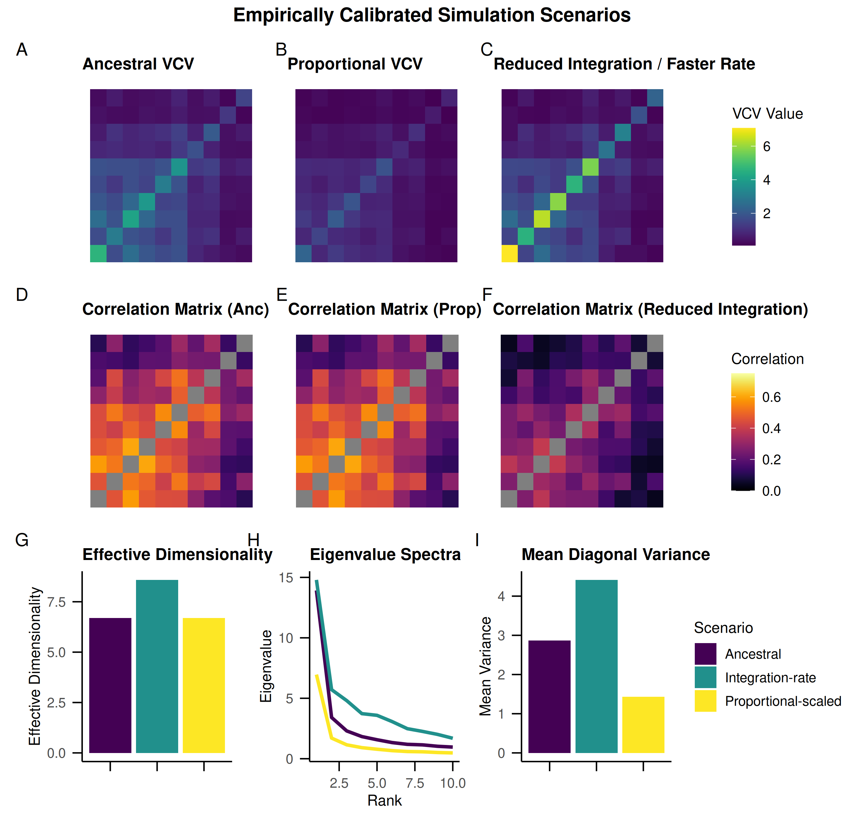
Figure 1. Empirically calibrated simulation scenarios. Panels A-C show the ancestral VCV, proportional scaling with s = 0.5, and a reduced-integration/faster-rate shift with g = 0.65. Panels D-F show their correlation matrices. Panels G-I summarize correlation effective dimensionality, covariance eigenvalue spectra, and mean marginal evolutionary variance. The proportional scenario changes scale without changing correlation structure; the integration-rate scenario changes covariance shape and rate together.
In the proportional panels, the covariance structure keeps the same shape and simply expands or contracts. In the integration-rate panels, weaker correlation structure is paired with larger marginal variance, so covariance shape and evolutionary rate change together. The shifted passerine examples below use these two simulation styles under repeated subtree resampling from the full tree, alongside a null no-shift baseline.
Before running simulations
Keep three practical details in mind.
Use the study function’s
seedargument for reproducibility. Do not pass a separate seed insidesimulation_options; the study functions manage replicate-level seeds.Study functions inherit template fit settings such as
methodanderror, so we explicitly overrideerrorfor simulated searches. Parallelize either the study or each search, not both; these examples run replicates in parallel and keep each search serial.Distinguish a successful search that finds no shifts from one with no eligible candidates or a failed fit. A successful zero-shift search is included in recovery evaluation: its true shifts count as missed. Check
per_replicate$n_candidates; with no candidates, recall can still be evaluated, but candidate-based specificity and false-positive rate are undefined for that replicate. Fitting failures are reported separately. The cutoff changes which nodes can be tested, not just the support required to accept a shift.
The next three sections show the individual study calls. The fixed-settings comparison then uses cached preview results to show the same logic side by side.
1. Estimate False Positives
The null study asks the baseline error question: if the real dataset contained no shifts at all, how often would the search still infer one?
# Estimate false positives under an empirical-covariance null model.
fp_study <- if (run_simulations) runFalsePositiveSimulationStudy(
  template = bodyplan_template,
  n_replicates = 500,
  tree_tip_count = 250,
  simulation_options = list(
    simulation_generator = "empirical"
  ),
  search_options = list(
    formula = "trait_data ~ 1",
    min_descendant_tips = 10,
    shift_acceptance_threshold = 10,
    IC = "GIC",
    num_cores = 1,
    method = "LL",
    error = FALSE,
    ic_uncertainty_threshold = 10,
    plot = FALSE,
    store_model_fit_history = FALSE
  ),
  num_cores = 8,
  seed = 5
)
# Inspect the study object, representative replicates, and aggregate summary.
if (run_simulations) {
  fp_study
  head(fp_study$per_replicate)
  fp_study$study_summary
}
Null simulations are useful for screening candidate choices of
shift_acceptance_threshold, IC, and
min_descendant_tips.
2. Estimate Recovery Under Proportional Scaling
Recovery under proportional scaling evaluates the scenario that
matches the current bifrost BMM search assumptions: shifted
covariance matrices are scalar multiples of the background covariance
matrix.
# Measure recovery when simulated shifts match proportional BMM scaling.
recovery_prop <- if (run_simulations) runShiftRecoverySimulationStudy(
  template = bodyplan_template,
  n_replicates = 500,
  tree_tip_count = 250,
  simulation_options = list(
    simulation_generator = "empirical",
    num_shifts = 5,
    min_shift_tips = 10,
    max_shift_tips = 40,
    scale_mode = "proportional",
    scale_factor_range = c(0.1, 2.0),
    exclude_range = c(0.5, 1.5),
    buffer = 3
  ),
  search_options = list(
    formula = "trait_data ~ 1",
    min_descendant_tips = 10,
    shift_acceptance_threshold = 10,
    IC = "GIC",
    num_cores = 1,
    method = "LL",
    error = FALSE,
    ic_uncertainty_threshold = 10,
    plot = FALSE,
    store_model_fit_history = FALSE
  ),
  fuzzy_distance = 2,
  weighted = TRUE,
  num_cores = 8,
  seed = 5
)
# Compare strict, fuzzy, and distance-weighted recovery summaries.
if (run_simulations) {
  recovery_prop
  recovery_prop$study_summary
  recovery_prop$evaluation$strict
  recovery_prop$evaluation$fuzzy
  recovery_prop$evaluation$weighted
}
3. Check the Integration-Rate Robustness Scenario
It is also useful to test a deliberately mismatched scenario in which
trait integration and evolutionary rate evolve together. This asks how
well the same search settings behave when the data depart from strict
proportional VCV scaling. The moderate power bands below sample reduced
integration from 0.5-0.8 and increased integration from
1.1-1.25; each power g scales marginal
variances by exactly 1 / g.
# Stress-test the same search under integration-rate model misspecification.
recovery_integration <- if (run_simulations) runShiftRecoverySimulationStudy(
  template = bodyplan_template,
  n_replicates = 500,
  tree_tip_count = 250,
  simulation_options = list(
    simulation_generator = "empirical",
    num_shifts = 5,
    min_shift_tips = 10,
    max_shift_tips = 40,
    scale_mode = "correlation",
    integration_power_range = c(0.5, 1.25),
    integration_exclude_range = c(0.8, 1.1),
    buffer = 3
  ),
  search_options = list(
    formula = "trait_data ~ 1",
    min_descendant_tips = 10,
    shift_acceptance_threshold = 10,
    IC = "GIC",
    num_cores = 1,
    method = "LL",
    error = FALSE,
    ic_uncertainty_threshold = 10,
    plot = FALSE,
    store_model_fit_history = FALSE
  ),
  fuzzy_distance = 2,
  weighted = TRUE,
  num_cores = 8,
  seed = 5
)
# Review the overall study and the fuzzy recovery result used for reporting.
if (run_simulations) {
  recovery_integration
  recovery_integration$study_summary
  recovery_integration$evaluation$fuzzy
}
This scenario changes covariance shape while the fitted search model permits only proportional covariance shifts. It therefore explores robustness to model misspecification. Recovery also depends on the magnitudes of the simulated rate changes, which differ between these scenarios; the comparison does not isolate the effect of covariance shape alone.
4. Compare Fixed Settings Across Scenarios
We now compare GIC and BIC at the same fixed settings across the null, proportional, and integration-rate scenarios. The saved results use 500 datasets per scenario, each based on a freshly resampled 250-tip subtree of the passerine tree with 12 simulated response traits.
The comparison holds shift_acceptance_threshold = 10 and
min_descendant_tips = 10. Each shifted dataset contains
five planted shifts in clades with 10 to 40 descendant tips. These
settings illustrate performance before tuning; Part 2 compares them with
more restrictive settings on the same datasets.
The individual calls above demonstrate each study separately. The saved tables instead extract the 10/10 settings from the paired grid in Part 2, where every setting is evaluated on the same datasets. Use that paired workflow and its reproduction scripts to reproduce these results; running the individual studies with their own seeds will generate different draws.
# Read the compact summaries without rerunning searches.
preview_tables <- readRDS(bifrost_example_file("simulation-preview-tables"))
fixed_settings_table <- preview_tables$fixed_settings
Table 1 summarizes false positives under the null; Table 2 summarizes recovery in datasets with planted shifts.
Null FP (%) is the mean percentage of eligible candidate
nodes incorrectly assigned a shift. Null any FP (%) is the
percentage of null datasets with at least one inferred shift. All 500
searches per scenario and IC completed successfully, including searches
that inferred no shifts.
| IC | Null FP (%) | Null any FP (%) | Mean shifts |
|---|---|---|---|
| GIC | 0.116 | 6.4 | 0.07 |
| BIC | 0.007 | 0.4 | 0.00 |
| IC | Scenario | Fuzzy rec. | Fuzzy spec. | Fuzzy F1 | Fuzzy BA | Mean shifts |
|---|---|---|---|---|---|---|
| GIC | Proportional | 0.849 | 0.985 | 0.845 | 0.917 | 5.05 |
| GIC | Integration-rate | 0.694 | 0.971 | 0.693 | 0.833 | 5.02 |
| BIC | Proportional | 0.788 | 0.989 | 0.829 | 0.888 | 4.50 |
| BIC | Integration-rate | 0.616 | 0.982 | 0.683 | 0.799 | 4.02 |
Because unshifted candidate nodes usually outnumber true shifts, raw accuracy can look high even when recovery is poor. Balanced accuracy gives recall and specificity equal weight; F1 instead combines precision and recall. Fuzzy scoring credits nearby inferred shifts as matches, allowing for uncertainty in their exact location.
For GIC, fuzzy balanced accuracy is 0.917 under proportional shifts and 0.833 under the integration-rate trade-off. The corresponding BIC values are 0.888 and 0.799. GIC recovers more shifts at these settings, but also infers shifts more often under the null. Part 2 shows how that trade-off affects the choice of search settings.
Performance Summary
These checks illustrate false-positive behavior and shift recovery under the simulated conditions, rather than establishing settings that will work for every dataset. Part 2 expands this fixed-setting comparison into a paired tuning grid on the same datasets and shows how to use the selected settings in an empirical search.
References
If you use these data or reproduce this workflow, the most relevant citations are:
- Berv, Jacob S., Charlotte M. Probst, Santiago Claramunt, J. Ryan Shipley, Matt Friedman, Stephen A. Smith, David F. Fouhey, and Brian C. Weeks. 2026. “Rates of passerine body plan evolution in time and space.” Nature Ecology & Evolution. https://doi.org/10.1038/s41559-026-03110-5
- Berv, Jacob S., Charlotte M. Probst, Santiago Claramunt, J. Ryan Shipley, Matt Friedman, Stephen A. Smith, David F. Fouhey, and Brian C. Weeks. 2026. “Supplementary data archive for Rates of passerine body plan evolution in time and space” (v1.0.0) [Data set]. Zenodo. https://doi.org/10.5281/zenodo.19198393
- Clavel, Julien, Laurent Aristide, and Helene Morlon. 2019. “A penalized likelihood framework for high-dimensional phylogenetic comparative methods and an application to New-World monkeys brain evolution.” Systematic Biology 68(1):93-116. https://doi.org/10.1093/sysbio/syy045
- Clavel, Julien, and Helene Morlon. 2020. “Reliable phylogenetic regressions for multivariate comparative data: Illustration with the MANOVA and application to the effect of diet on mandible morphology in phyllostomid bats.” Systematic Biology 69(5):927-943. https://doi.org/10.1093/sysbio/syaa010
- Clavel, Julien, Gilles Escarguel, and Gildas Merceron. 2015. “mvMORPH: an R package for fitting multivariate evolutionary models to morphometric data.” Methods in Ecology and Evolution 6(11):1311-1319. https://doi.org/10.1111/2041-210X.12420
- Smith, Stephen A., Nicholas Walker-Hale, and Caroline T. Parins-Fukuchi. 2023. “Compositional shifts associated with major evolutionary transitions in plants.” New Phytologist 239(6):2404-2415. https://doi.org/10.1111/nph.19099
Software Used in This Vignette
-
bifrostfor empirical simulation templates, null and shifted datasets, repeated simulation studies, recovery evaluation, and tuning-grid summaries. -
mvMORPH/mvglsmachinery underlies the global calibration fit and empirical shift searches. -
apeandphytoolsunderlie the phylogenetic tree, SIMMAP, and subtree operations used by the simulation helpers. -
ggplot2,patchwork, andviridisdraw the schematic simulation-scenario figure. -
knitrandrmarkdownrender the vignette and preview tables.