Passerine Body Plan Evolution, Part 4: Shift Magnitude Comparisons • bifrost

Introduction

Berv et al. (2026) used bifrost to identify hidden rate shifts in multivariate skeletal evolution across the passerine tree. Part 4 asks what those accepted parent-child regime changes imply about direction and magnitude: when the model infers a rate increase or decrease, how often does each direction occur, and how large are the changes?

Berv et al. (2026) reported this comparison in Supplementary Figure 5. Their workflow counted rate-increase and rate-decrease shifts within each sensitivity run, then pooled inferred shifts across the 12 temporal sensitivity searches. The pooled shifts were summarized three ways: GIC and BIC runs together, GIC runs only, and BIC runs only.

This vignette computes that non-spatial shift-magnitude workflow from compact package data. Parts 1-3 introduce the focal search, lineage-rate summaries, and transition table used here. We first show the single-run calculation on the focal min10.ic20.gic result, then load the compact sensitivity bundle to obtain the run-level shift-direction frequencies and pooled magnitude-density comparisons. The magnitude test compares log(abs(rate_delta)) for increases and decreases with a Monte-Carlo two-sample KS test.

Loading the compact focal result

Start with the compact focal result bundled with bifrost. This object represents the min10.ic20.gic search and keeps the final mapped tree plus fitted BMM regime rates.

# Load the focal min10.ic20.gic search used for the single-run example.
search_path <- system.file(
  "extdata",
  "avian-skeleton",
  "passerine_bodyplan_search_compact.RDS",
  package = "bifrost"
)
stopifnot(nzchar(search_path))

bodyplan_search <- readRDS(search_path)

# Preserve the S3 class if an older serialized copy lacks it.
if (!inherits(bodyplan_search, "bifrost_search")) {
  class(bodyplan_search) <- c("bifrost_search", class(bodyplan_search))
}

# Confirm that the compact object has the fitted BMM regimes and shifts.
data.frame(
  model = bodyplan_search$model_no_uncertainty$model,
  fitted_regimes = length(bodyplan_search$model_no_uncertainty$param),
  accepted_shifts = length(bodyplan_search$shift_nodes_no_uncertainty)
)
#>   model fitted_regimes accepted_shifts
#> 1   BMM             83              82

Focal run: shift magnitudes

shift_transitions() extracts each inferred parent-child regime change and records the signed fitted rate difference in rate_delta. compare_shift_magnitudes() then follows the Berv et al. (2026) default comparison: it separates increases from decreases, transforms magnitudes as log(abs(rate_delta)), and runs a two-sample KS test.

# Extract accepted focal shifts, excluding the root state assignment.
bodyplan_transitions <- shift_transitions(bodyplan_search, include_root = FALSE)

# Count rate increases and decreases before testing magnitudes.
shift_magnitude_counts(bodyplan_transitions)
#>   source decrease increase total decrease_frequency increase_frequency
#> 1  input       64       18    82          0.7804878          0.2195122

# Preview the signed and percentage rate-change columns used below.
head(bodyplan_transitions[, c(
  "node",
  "parent_rate",
  "child_rate",
  "rate_delta",
  "percentage_change",
  "rate_change"
)])
#>   node  parent_rate   child_rate    rate_delta percentage_change rate_change
#> 1 3620 0.0325232187 0.0005337094 -0.0319895094         -98.35899    decrease
#> 2 2059 0.0325232187 0.0028624293 -0.0296607895         -91.19881    decrease
#> 3 2060 0.0028624293 0.0003045813 -0.0025578479         -89.35934    decrease
#> 4 4105 0.0005337094 0.0001172235 -0.0004164859         -78.03609    decrease
#> 5 2065 0.0003045813 0.0008134411  0.0005088598         167.06861    increase
#> 6 2837 0.0008134411 0.0002988457 -0.0005145954         -63.26155    decrease

# Fix the seed because the KS p-value uses Monte-Carlo simulation.
set.seed(1)
bodyplan_magnitude_test <- compare_shift_magnitudes(
  bodyplan_transitions,
  ks_reps = 10000
)

# Extract the compact result tables most useful for inspection.
magnitude_summary <- as.data.frame(bodyplan_magnitude_test, component = "summary")
magnitude_tests <- as.data.frame(bodyplan_magnitude_test, component = "tests")
magnitude_modes <- as.data.frame(bodyplan_magnitude_test, component = "modal")

print(magnitude_summary)
#>   rate_change  n   mean median mean_abs_raw median_abs_raw
#> 1    increase 18 -7.796 -7.846     0.001105      0.0003936
#> 2    decrease 64 -7.988 -8.396     0.001664      0.0002257
cat("\n\n")
print(magnitude_tests)
#>   test statistic p_value mean_difference median_difference
#> 1   ks    0.1736  0.7149          0.1916            0.5503
#>                                           method
#> 1 Monte-Carlo two-sample Kolmogorov-Smirnov test
cat("\n\n")
print(magnitude_modes)
#>   mode_increase mode_decrease mode_difference linear_ratio
#> 1        -7.795        -8.738          0.9425        2.566

The modal summary gives the KDE-estimated mode for each transformed magnitude distribution. On the default log-absolute scale, linear_ratio back-transforms those modes and reports the inferred increase-magnitude mode divided by the inferred decrease-magnitude mode.

The focal KS table is a single-run teaching example for min10.ic20.gic; it is not the pooled sensitivity test reported for Supplementary Figure 5. Those pooled KS values are computed below after grouping all 12 sensitivity runs. The same function can also run the simpler Welch t-test and Wilcoxon comparisons from the Berv et al. (2026) utility code by setting transform = "absolute" and tests = c("t", "wilcox").

Sensitivity runs: pooled inputs

The focal run demonstrates the mechanics, but Supplementary Figure 5 pools shifts across the Berv et al. (2026) sensitivity analyses. The pooled workflow has two outputs: run-level increase/decrease frequencies and pooled magnitude-density comparisons. Both start from the same compact sensitivity bundle.

Load the compact sensitivity bundle

The bundle contains reduced versions of the 12 Berv et al. (2026) search outputs, one for each combination of minimum clade size, IC acceptance threshold, and information criterion. Each object keeps the final mapped tree and fitted BMM regime rates needed for transition extraction.

# Load the compact bundle of all 12 temporal sensitivity searches.
sensitivity_path <- system.file(
  "extdata",
  "avian-skeleton",
  "passerine_bodyplan_search_sensitivity_compact.RDS",
  package = "bifrost"
)
stopifnot(nzchar(sensitivity_path))

bodyplan_sensitivity_searches <- readRDS(sensitivity_path)

# Report bundle size and run-label coverage for orientation.
data.frame(
  sensitivity_runs = length(bodyplan_sensitivity_searches),
  compressed_size_mb = round(file.info(sensitivity_path)$size / 1024^2, 2),
  first_run = names(bodyplan_sensitivity_searches)[1],
  last_run = tail(names(bodyplan_sensitivity_searches), 1)
)
#>   sensitivity_runs compressed_size_mb      first_run       last_run
#> 1               12               0.38 min30.ic40.gic min10.ic20.bic

Extract transitions and define analysis groups

Each sensitivity run is converted to the same transition-table representation used for the focal run. We then define the three pooled groups used in Supplementary Figure 5: all GIC and BIC runs together, GIC runs only, and BIC runs only.

# Extract transitions from each sensitivity run with the same rule as the focal run.
bodyplan_sensitivity_transitions <- lapply(
  bodyplan_sensitivity_searches,
  shift_transitions,
  include_root = FALSE
)

# Count increase/decrease frequencies for every run.
sensitivity_shift_counts <- shift_magnitude_counts(
  bodyplan_sensitivity_transitions
)

sensitivity_shift_counts
#>            source decrease increase total decrease_frequency increase_frequency
#> 1  min30.ic40.gic       11        7    18          0.6111111          0.3888889
#> 2  min30.ic40.bic        6        7    13          0.4615385          0.5384615
#> 3  min20.ic40.gic       11        6    17          0.6470588          0.3529412
#> 4  min20.ic40.bic        9        7    16          0.5625000          0.4375000
#> 5  min10.ic40.gic       16        9    25          0.6400000          0.3600000
#> 6  min10.ic40.bic       13        9    22          0.5909091          0.4090909
#> 7  min30.ic20.gic       25        7    32          0.7812500          0.2187500
#> 8  min30.ic20.bic       21        7    28          0.7500000          0.2500000
#> 9  min20.ic20.gic       33       12    45          0.7333333          0.2666667
#> 10 min20.ic20.bic       27        7    34          0.7941176          0.2058824
#> 11 min10.ic20.gic       64       18    82          0.7804878          0.2195122
#> 12 min10.ic20.bic       42       14    56          0.7500000          0.2500000

Shift-direction frequencies across runs

Before comparing magnitudes, Berv et al. (2026) compared how often inferred shifts increased or decreased rates within each sensitivity run. shift_magnitude_groups() makes the grouped analysis explicit; shift_magnitude_counts() then returns one count table per named group. Select one count table with [[ ]], then call plot().

# Draw one paired-frequency panel for each pooled analysis set.
bodyplan_frequency_plot_results <- list()

bodyplan_frequency_plot_results[["GIC + BIC"]] <- plot(
  pooled_shift_counts[["GIC + BIC"]],
  statistic = "frequency",
  main = "GIC + BIC",
  ylim = c(0, 1)
)

bodyplan_frequency_plot_results[["GIC"]] <- plot(
  pooled_shift_counts[["GIC"]],
  statistic = "frequency",
  main = "GIC",
  ylim = c(0, 1)
)

bodyplan_frequency_plot_results[["BIC"]] <- plot(
  pooled_shift_counts[["BIC"]],
  statistic = "frequency",
  main = "BIC",
  ylim = c(0, 1)
)

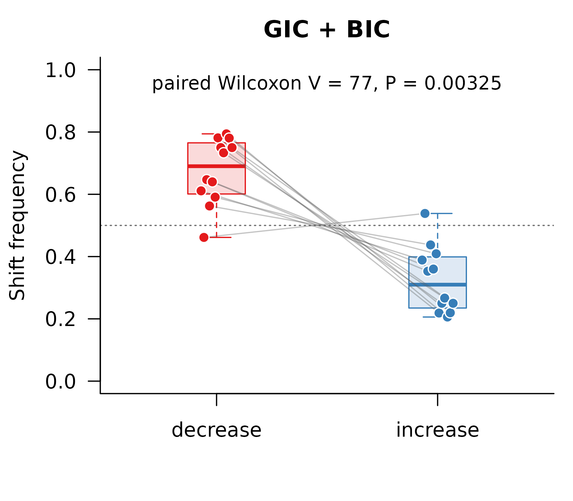
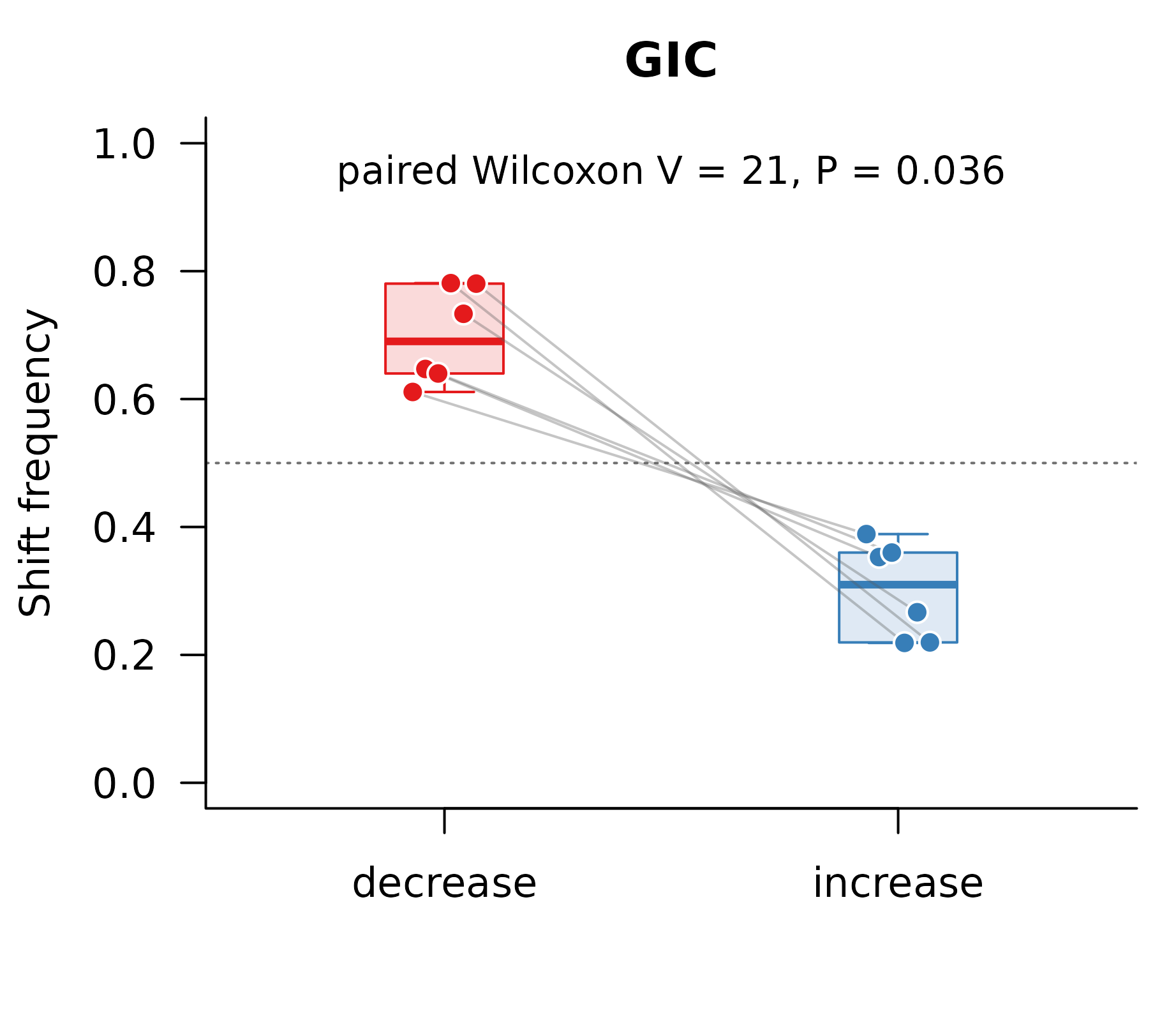
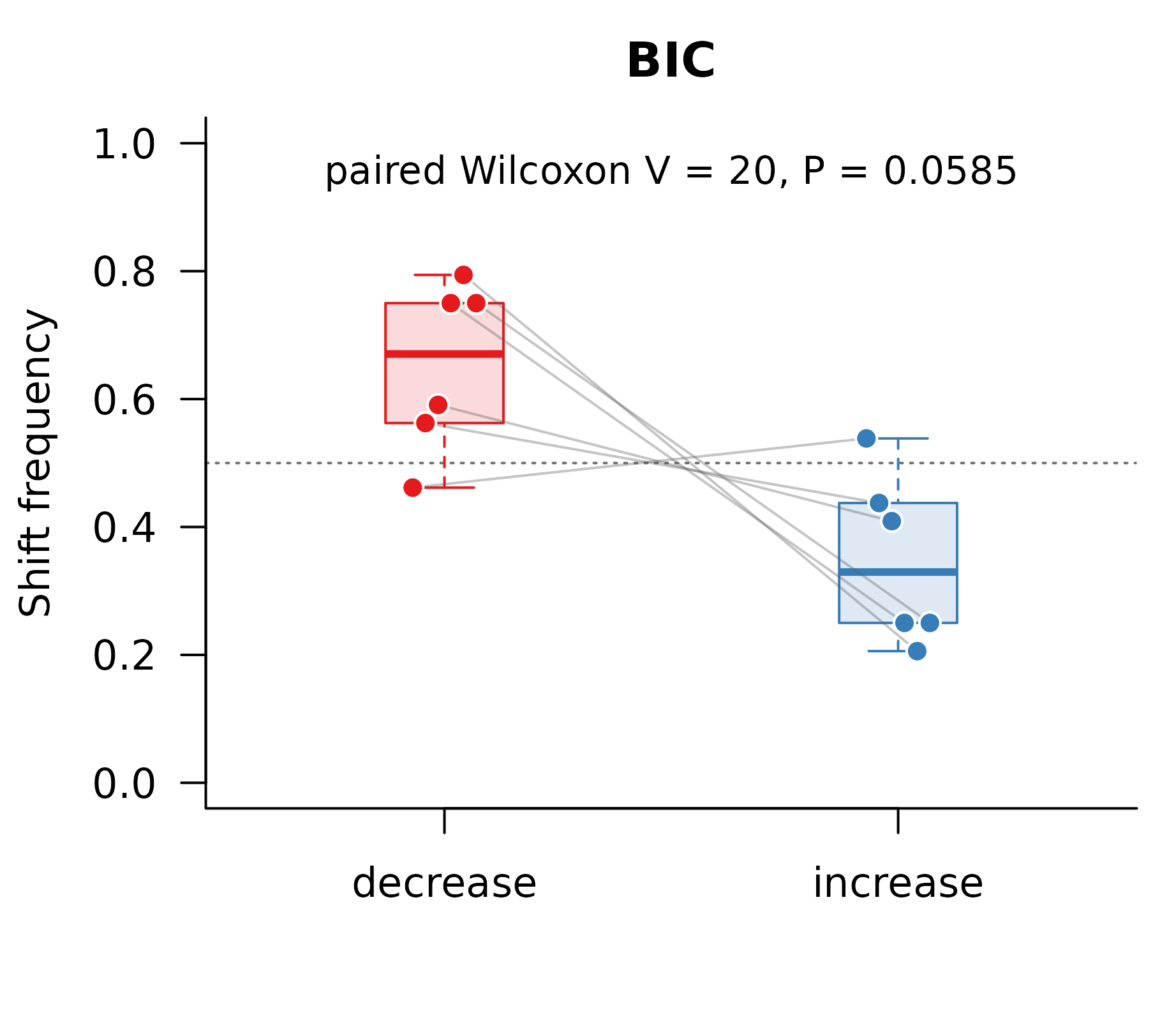
**Figure 1. Shift-direction frequencies across sensitivity analyses.** Left, middle, and right panels show the pooled GIC + BIC, GIC-only, and BIC-only analysis sets. Lines connect paired decrease and increase frequencies from the same search output; the dashed line marks equal increase and decrease frequencies.

Figure 1. Shift-direction frequencies across sensitivity analyses. Left, middle, and right panels show the pooled GIC + BIC, GIC-only, and BIC-only analysis sets. Lines connect paired decrease and increase frequencies from the same search output; the dashed line marks equal increase and decrease frequencies.

The numerical test rows returned by plot() reproduce the paired Wilcoxon signed-rank tests shown in the Supplementary Figure 5 frequency panels. mean_difference is the paired mean of increase_frequency - decrease_frequency, so negative values indicate that decreases are more frequent.

# Combine the three paired-frequency test tables into one report.
bodyplan_frequency_tests <- do.call(
  rbind,
  list(
    bodyplan_frequency_plot_results[["GIC + BIC"]]$tests,
    bodyplan_frequency_plot_results[["GIC"]]$tests,
    bodyplan_frequency_plot_results[["BIC"]]$tests
  )
)

# Retain the sample sizes, test statistics, and directional effect summary.
bodyplan_frequency_tests <- bodyplan_frequency_tests[
  ,
  c(
    "analysis",
    "n",
    "wilcox_statistic",
    "wilcox_p_value",
    "mean_difference"
  )
]
rownames(bodyplan_frequency_tests) <- NULL

# Format inferential results for compact display.
bodyplan_frequency_tests$wilcox_p_value <- signif(
  bodyplan_frequency_tests$wilcox_p_value,
  4
)
bodyplan_frequency_tests$mean_difference <- round(
  bodyplan_frequency_tests$mean_difference,
  4
)

print(bodyplan_frequency_tests)
#>    analysis  n wilcox_statistic wilcox_p_value mean_difference
#> 1 GIC + BIC 12               77       0.003252         -0.3504
#> 2       GIC  6               21       0.036030         -0.3977
#> 3       BIC  6               20       0.058480         -0.3030

Pooled magnitude comparisons

The second pooled output compares the magnitudes of rate increases and decreases after pooling shifts within each analysis group. Because pooled_transition_groups is a grouped object, compare_shift_magnitudes() applies the same KS comparison to each named group and returns a named comparison set. The call below keeps the random seed fixed because the simulated KS p-values and bootstrap mean p-values use Monte-Carlo resampling.

Run the pooled KS tests

# Fix the seed for simulated KS p-values and bootstrap summaries.
set.seed(2026)

# Run the same magnitude comparison for each pooled analysis set.
pooled_magnitude_comparisons <- compare_shift_magnitudes(
  pooled_transition_groups,
  ks_reps = 10000,
  bootstrap_p_value = TRUE,
  bootstrap_reps = 100
)

# Extract one compact KS-test table for the grouped comparison.
as.data.frame(pooled_magnitude_comparisons, component = "ks")
#>    analysis increases decreases   ks_D   ks_p bootstrap_mean_p mode_increase
#> 1 GIC + BIC       110       278 0.2396 0.0002          0.01064        -7.821
#> 2       GIC        59       160 0.2405 0.0104          0.06137        -7.866
#> 3       BIC        51       118 0.2340 0.0338          0.08272        -7.793
#>   mode_decrease linear_ratio
#> 1        -8.836        2.762
#> 2        -8.793        2.527
#> 3        -8.865        2.920

Plot frequency-scaled magnitude densities

The plot() method for a shift_magnitude_comparison object draws Supplementary Figure 5-style density panels. The default scale_by_frequency = TRUE matches the Berv et al. (2026) plotting logic by scaling each density by the observed frequency of that shift direction. Each call draws one selected comparison, so the same [[ ]] pattern used for count plots applies here.

# Plot one frequency-scaled density panel for each pooled comparison.
plot(
  pooled_magnitude_comparisons[["GIC + BIC"]],
  main = "GIC + BIC",
  legend = FALSE,
  xlim = c(-10.5, -5),
  ylim = c(0, 0.4)
)

plot(
  pooled_magnitude_comparisons[["GIC"]],
  main = "GIC",
  legend = FALSE,
  xlim = c(-10.5, -5),
  ylim = c(0, 0.4)
)

plot(
  pooled_magnitude_comparisons[["BIC"]],
  main = "BIC",
  legend = FALSE,
  xlim = c(-10.5, -5),
  ylim = c(0, 0.4)
)

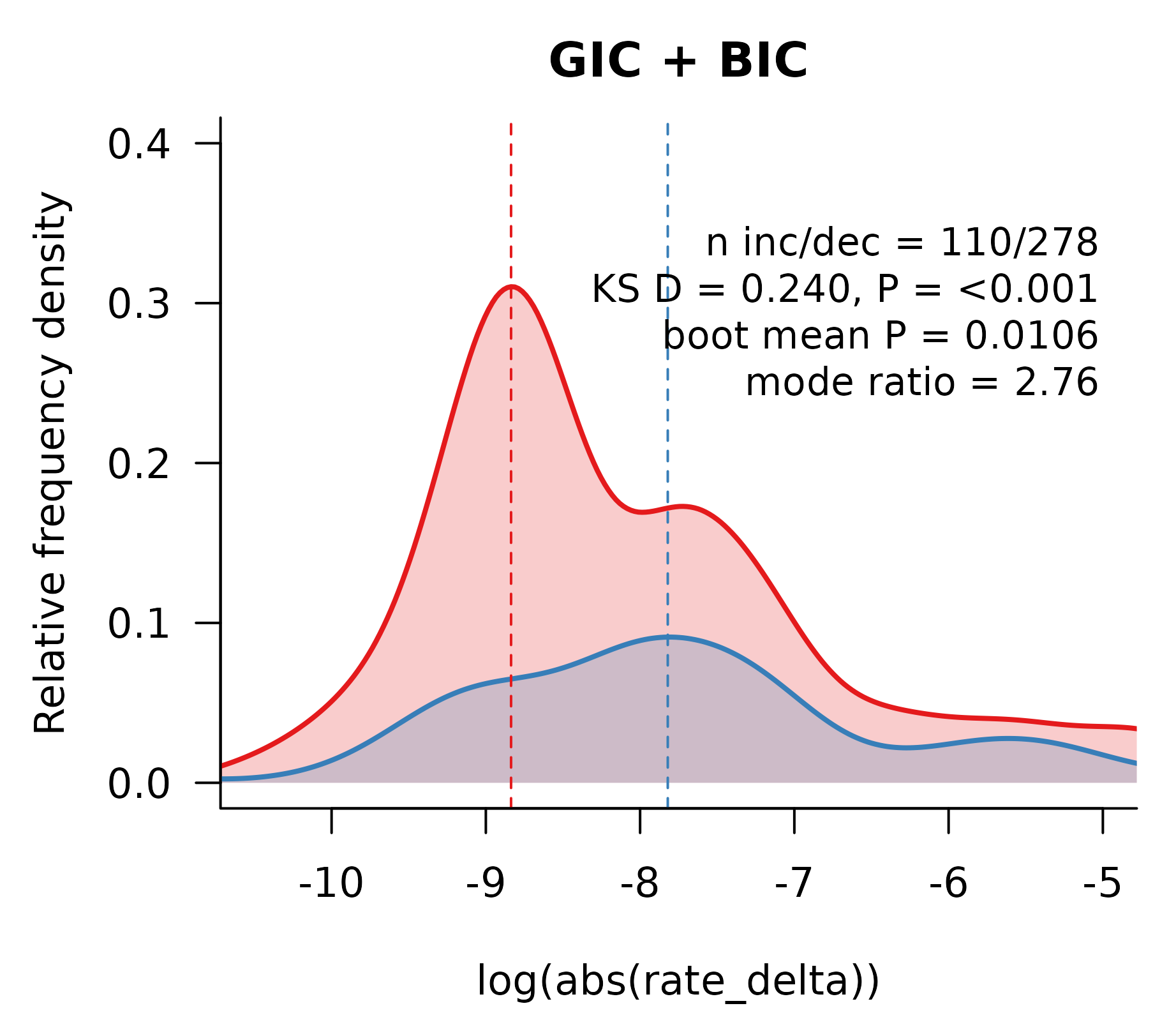
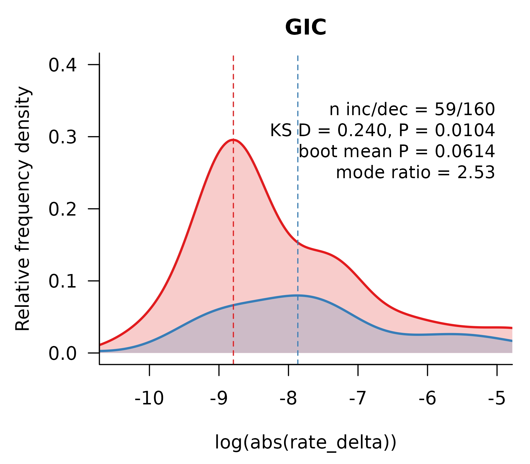
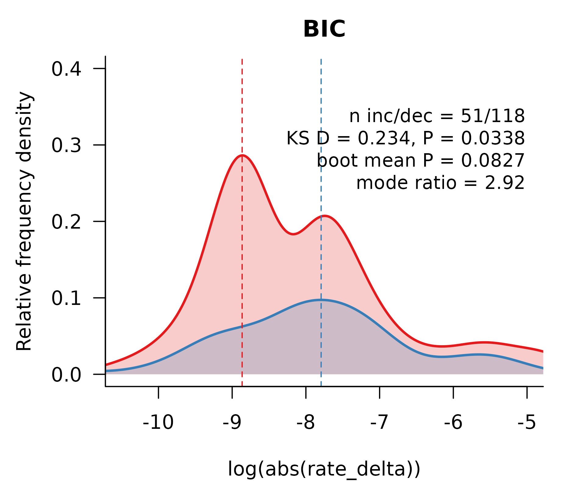
**Figure 2. Log absolute rate-delta magnitude distributions.** Left, middle, and right panels show the pooled GIC + BIC, GIC-only, and BIC-only analysis sets. Red curves show decreases and blue curves show increases. Densities integrate to observed shift-direction frequencies across the Berv et al. (2026) sensitivity analyses; dashed vertical lines mark KDE modes.

Figure 2. Log absolute rate-delta magnitude distributions. Left, middle, and right panels show the pooled GIC + BIC, GIC-only, and BIC-only analysis sets. Red curves show decreases and blue curves show increases. Densities integrate to observed shift-direction frequencies across the Berv et al. (2026) sensitivity analyses; dashed vertical lines mark KDE modes.

The compact sensitivity bundle yields the local sample sizes, KS statistics, KDE modes, and back-transformed modal ratios used in these pooled comparisons. Use the full Zenodo archive for proposal-level history, sensitivity searches, and full workflow verification.

Across the pooled sensitivity summaries, inferred decreases are more frequent than increases. The magnitude-density panels show the complementary pattern: the KDE modes for rate increases fall at larger log(abs(rate_delta)) values than the modes for decreases, so the modal increase magnitude is larger after back-transformation.

The KS p-values and bootstrap mean p-values use Monte-Carlo simulation, so repeated runs can differ slightly unless you set the random seed. Increase bootstrap_reps if you want a more stable bootstrap mean p-value.

If you want to start from the complete Berv et al. (2026) archive instead of the compact bundle, load the same 12 search RDS files from data/temporal/02_shift_search/new_bifrost/, wrap the named analysis sets with shift_magnitude_groups(), and pass that object to shift_magnitude_counts() or compare_shift_magnitudes().

Practical Takeaways

shift_transitions() turns fitted BMM regime changes into an explicit transition table with parent rates, child rates, signed rate deltas, and increase/decrease labels.
shift_magnitude_groups() marks named analysis sets that should be analyzed separately rather than pooled into one result.
shift_magnitude_counts() computes run-level increase/decrease counts and frequencies for one analysis set or each group in a shift_magnitude_groups object.
compare_shift_magnitudes() compares log absolute rate-change magnitudes for one pooled set or each group in a shift_magnitude_groups object.
as.data.frame() extracts compact count, summary, test, modal, and pooled KS tables from the count and comparison objects.
plot() draws one selected count or magnitude-comparison object at a time.
The compact sensitivity bundle yields the local Supplementary Figure 5-style shift-magnitude summaries without requiring the 15.2 GB Berv et al. (2026) archive.
Use the complete Berv et al. (2026) archive when you need proposal-level history, sensitivity searches, full workflow verification, or the full fitted candidate models.
Continue to Part 5 for the temporal post-hoc integration workflow behind Supplementary Text 2.1 and Supplementary Figure 4.

References

If you use these data or reproduce this workflow, the most relevant citations are:

Berv, Jacob S., Charlotte M. Probst, Santiago Claramunt, J. Ryan Shipley, Matt Friedman, Stephen A. Smith, David F. Fouhey, and Brian C. Weeks. 2026. “Rates of passerine body plan evolution in time and space.” Nature Ecology & Evolution. https://doi.org/10.1038/s41559-026-03110-5
Berv, Jacob S., Charlotte M. Probst, Santiago Claramunt, J. Ryan Shipley, Matt Friedman, Stephen A. Smith, David F. Fouhey, and Brian C. Weeks. 2026. “Supplementary data archive for Rates of passerine body plan evolution in time and space” (v1.0.0) [Data set]. Zenodo. https://doi.org/10.5281/zenodo.19198393
Claramunt, Santiago, Christopher Sheard, Joseph W. Brown, Guillermo Cortes-Ramirez, Joel Cracraft, Mason M. Su, Brian C. Weeks, and Joseph A. Tobias. 2025. “A new time tree of birds reveals the interplay between dispersal, geographic range size, and diversification.” Current Biology. Advance online publication. https://doi.org/10.1016/j.cub.2025.07.004

Software Used in This Vignette

bifrost for transition extraction and shift-magnitude comparisons.
ape and phytools underlie the mapped-tree calculations in these summaries.

AI Assistance

This vignette was developed with assistance from OpenAI tools for drafting, editing, and figure refinement; all scientific content, interpretation, and final decisions were reviewed by the authors.