Mapping Sensitivity in Jaw-Shape Evolutionary Rates with rateMap, Part 2 • bifrost

Overview

Part 1 built the core equal-weight rateMap() workflow: load a cached threshold sweep, inspect the first-pass fitted-rate range, and then display effectively zero-rate branches with explicit near-zero metadata. This second part starts from the same cached jaw-shape sweep and explores the extensions that are useful after the main map is stable.

As in Part 1, plotted rate categories are display bins over fitted branch summaries, not newly inferred bifrost regimes. Rate flags are diagnostic metadata used for display; they do not remove branches or change fitted values.

Read Part 1: Workflow and near-zero diagnostics first if you want the setup and main equal-weight map.

Setup

Load the packages needed for the comparison and diagnostic views.

library(bifrost)
library(ape)
library(phytools)

Load the reference tree used for plotting and same-topology examples.

tree_path <- system.file(
  "extdata", "jaw-shape", "mrbayes_prune_tree.RDS",
  package = "bifrost"
)
fish.tree <- readRDS(tree_path)
fish.tree <- ladderize(untangle(as.phylo(fish.tree)))

Load the cached threshold sweep created in Part 1.

cache_path <- rate_map_cache_path()
if (!file.exists(cache_path)) {
  stop("No jaw-shape threshold cache found; run the Part 1 sweep first.")
}
jaw_threshold_runs <- readRDS(cache_path)
threshold_grid <- as.numeric(sub("GIC_threshold_", "", names(jaw_threshold_runs)))

Reconstruct the adjusted equal-weight object from Part 1 so uncertainty maps and branch-level diagnostics in this part have the same Otsu-style tail-cluster near-zero metadata, adapted from Otsu’s histogram thresholding criterion (Otsu 1979).

jaw_rate_map_equal <- rateMap(
  jaw_threshold_runs,
  weights = "equal",
  uncertainty = TRUE,
  progress = TRUE,
  control = rateMapControl(
    rate_flags = rateMapRateFlags(method = "tail_cluster")
  )
)
jaw_rate_map_equal <- rateMapView(
  jaw_rate_map_equal,
  palette = "Viridis",
  legend_title = "Mean log fitted rate"
)

IC-Weighted Rate Map

An IC-weighted map asks a different question: which log-rate pattern is emphasized when lower-GIC threshold outcomes contribute more heavily?

Use this view when the threshold-generated fits form a small set of comparable model outcomes. All retained runs must use the same IC family, so do not mix GIC and BIC runs in a single weights = "ic" map. If one threshold dominates the IC weights, the result will resemble that single model more than an across-threshold robustness summary. In a threshold sweep, this can favor a more permissive fitted configuration, so read the map as a model-outcome weighting over retained fits rather than as a formal threshold-selection rule.

jaw_rate_map_ic <- rateMap(
  jaw_threshold_runs,
  weights = "ic",
  uncertainty = TRUE,
  progress = TRUE,
  control = rateMapControl(
    rate_flags = rateMapRateFlags(method = "tail_cluster")
  )
)
jaw_rate_map_ic <- rateMapView(
  jaw_rate_map_ic,
  palette = "Viridis",
  legend_title = "IC-weighted mean log fitted rate"
)

jaw_rate_map_ic
jaw_rate_map_ic$weight_table
jaw_rate_map_ic$rate_categories

#> rateMap object
#> - fits: 6
#> - summary: branch
#> - target: first
#> - check: full
#> - weights: ic
#> - uncertainty: TRUE
#> - color mode: category
#> - plotted value: value
#> - value range: -25.79 to -11.36
#> - rate flags: 54 near-zero, 0 high-outlier (method: tail_cluster)
#> - fold range: 1857530 full, 714 regular
#> - sd range: 0.005051 to 0.665

input_index	weight	ic	IC_used
3	0.952	-342739.4	GIC
5	0.04798	-342733.4	GIC
1	2.498e-27	-342617.0	GIC
2	5.760e-46	-342531.2	GIC
4	1.761e-62	-342455.1	GIC
6	1.887e-72	-342409.2	GIC

Table 1. IC weights. Relative fit weights used in the IC-weighted branch-category map. input_index identifies the retained search in the input list; weight is the normalized IC weight used by rateMap(); ic is the selected model’s IC value; and IC_used records the criterion used to compute comparable weights. In this sweep, inputs 3 and 5 carry nearly all of the IC weight, while the other retained runs have effectively zero weight.

rate_category	n_branches	value_mean	value_median	value_sd	total_branch_length
near-zero	54	-21.94	-21.67	1.113	388.1
-18 to -17	8	-17.93	-17.93	0	107.4
-17 to -16	6	-16.23	-16.1	0.1875	33.21
-16 to -15	48	-15.37	-15.08	0.3215	312.1
-15 to -14	0	NA	NA	NA	0
-14 to -13	12	-13.26	-13.26	0	110.5
-13 to -12	20	-12.36	-12.3	0.1794	132.2
-12 to -11	22	-11.36	-11.36	0	126.6

Table 2. IC-weighted rate categories. Condensed ordered log-rate bins used to color the IC-weighted branch-category map. rate_category is the displayed interval or diagnostic class; n_branches counts branches assigned to the bin; value_mean, value_median, and value_sd summarize plotted branch log-rates; and total_branch_length gives the summed branch length in that displayed bin. The full generated category table remains available as rate_map_ic_categories.csv.

plot(
  jaw_rate_map_ic,
  type = "arc",
  show_tip_labels = FALSE,
  legend_fsize = 0.9,
  arc_height = 0.5
)

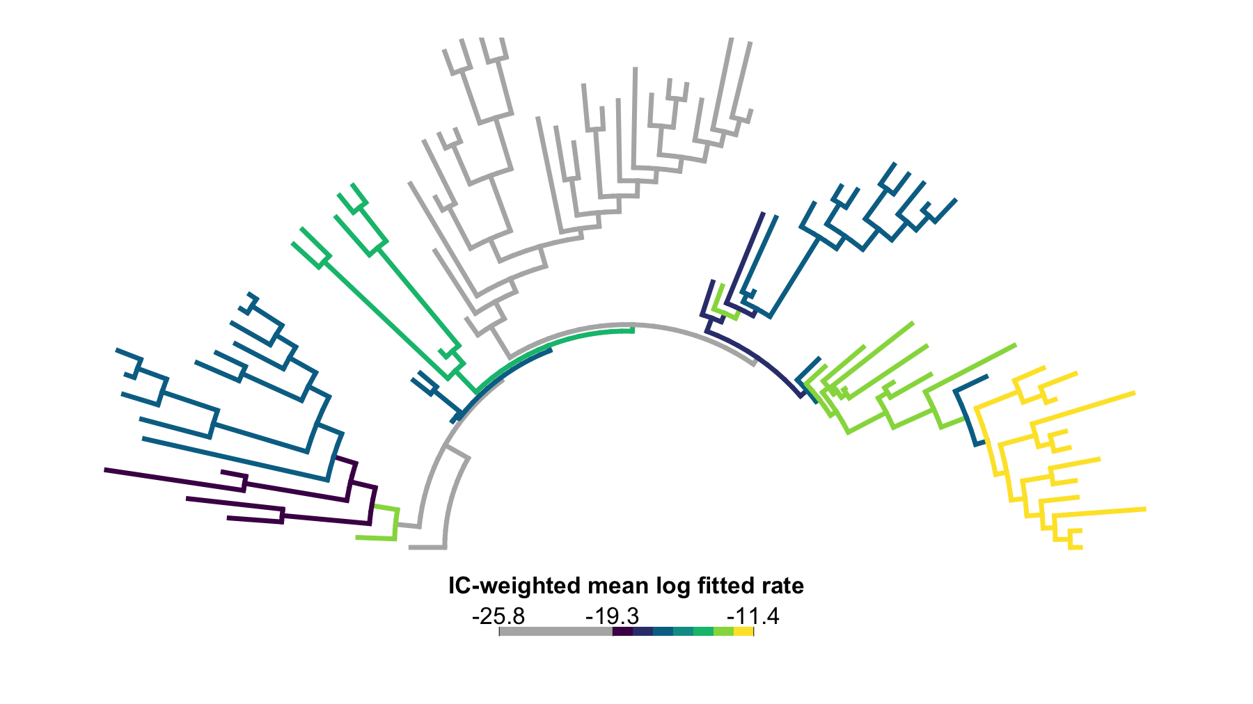
Arc-style phylogenetic tree with grey near-zero branches and colored IC-weighted branch log-rate categories across the jaw-shape threshold sweep.

Figure 1. IC-weighted branch-category rate map after near-zero flagging. This arc tree summarizes the same threshold sweep after weighting each completed search by its relative GIC support. Branches in the separated lower log-rate cluster are shown as a separate grey category; remaining regular branches are colored by ordered categories of the IC-weighted mean fitted log-rate.

Here the IC weights concentrate on thresholds 20 and 30, with threshold 20 carrying most of the weight. The weighting choice does not change the log-rate scale; weights = "ic" changes only the fit-level weights in the weighted mean log-rate. The IC-weighted map is visually similar to the equal-weight map because the dominant lower-GIC searches preserve the same broad branch-rate structure. The maps are not identical: branch values are recomputed under IC weights, and some branches shift color categories, but the main high-rate regions remain stable. Appendix E shows the largest branch-level differences between weighting schemes.

Mapping Uncertainty Across Thresholds

With uncertainty = TRUE, rateMap() stores run-level log-rate values and adds branch-level summaries: weighted mean, weighted median, standard deviation, quantiles, highest-density interval bounds, and coefficient of variation. The highest-density interval contains 95% of the weighted run-level values by default; set control = list(highest_density_interval_prob = ...) to change that probability. For equal weights, sd is the ordinary sample standard deviation across runs; for IC or custom weights, it is computed from the normalized weighted variance. In this threshold sweep, these columns summarize variation across fitted searches. They do not measure landmark error, posterior tree uncertainty, or uncertainty inside the original fitted models. They also do not use the per-shift support weights that bifrost can compute inside an individual search; the weights here are the fit-level weights supplied to rateMap().

For the equal-weight six-run map shown here, the default 95% highest-density interval is deliberately conservative and effectively spans all retained run-level values for each branch. With denser run stacks, the same column behaves more like the familiar shortest interval containing the requested probability mass; for small sensitivity sweeps, interpret it as a range-like stability diagnostic.

You can recolor the same object by any compatible numeric column. For uncertainty summaries, continuous color ramps are often easier to read than discrete categories. The plotted summary table can still be sorted by sd or highest_density_interval_width for reporting, but the tree views are the most direct way to see where threshold sensitivity sits on the phylogeny. For Figures 2 and 3, color encodes uncertainty rather than rate magnitude; darker branches are more stable across the threshold sweep, while lighter branches vary more across runs. As a first example, plot the across-threshold standard deviation:

plot(
  jaw_rate_map_equal,
  value = "sd",
  type = "arc",
  show_tip_labels = FALSE,
  palette = "Inferno",
  color_mode = "continuous",
  legend_fsize = 0.9,
  arc_height = 0.5
)

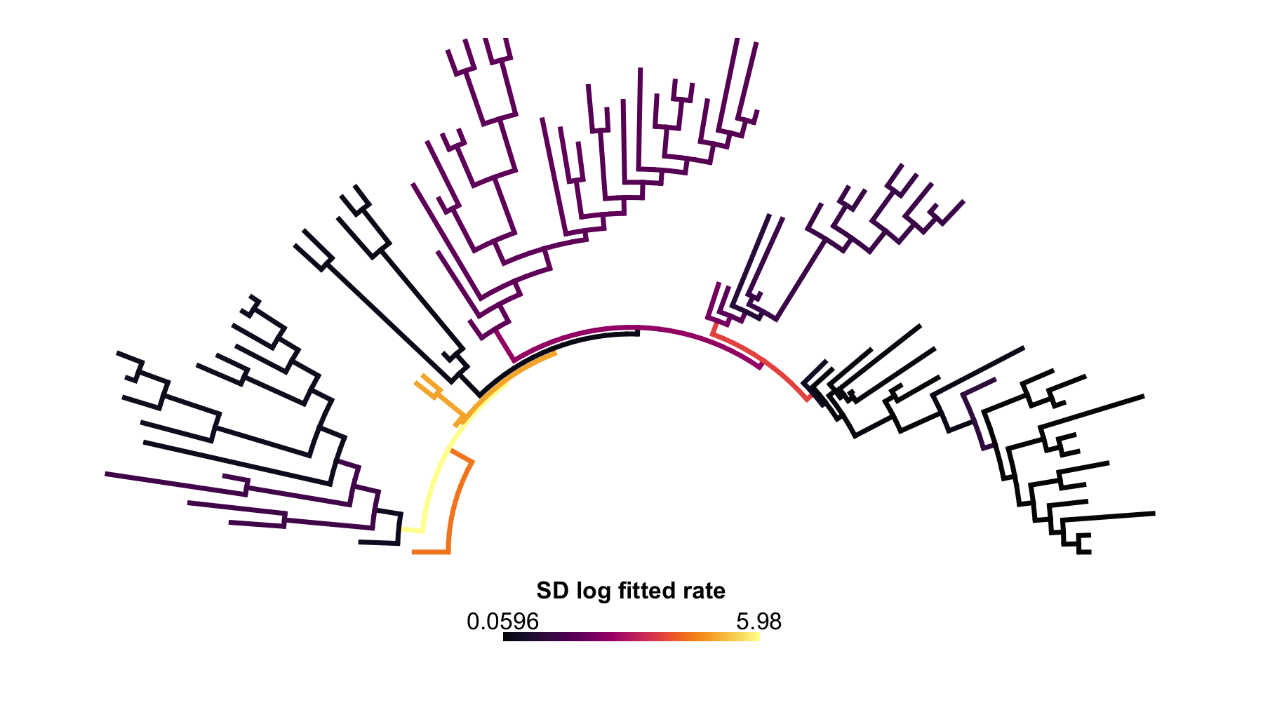
Arc-style phylogenetic tree with branches colored by across-threshold standard deviation in fitted log-rate.

Figure 2. Across-threshold standard deviation. This uncertainty map recolors the equal-weight rateMap() object by the standard deviation of fitted branch log-rates across the six threshold searches. Larger values mark branches whose inferred rates change more across the threshold sweep, while smaller values mark branches with more stable rate assignments.

Or plot the highest-density, or shortest weighted, interval width:

plot(
  jaw_rate_map_equal,
  value = "highest_density_interval_width",
  type = "arc",
  show_tip_labels = FALSE,
  palette = "Plasma",
  color_mode = "continuous",
  legend_fsize = 0.9,
  arc_height = 0.5
)

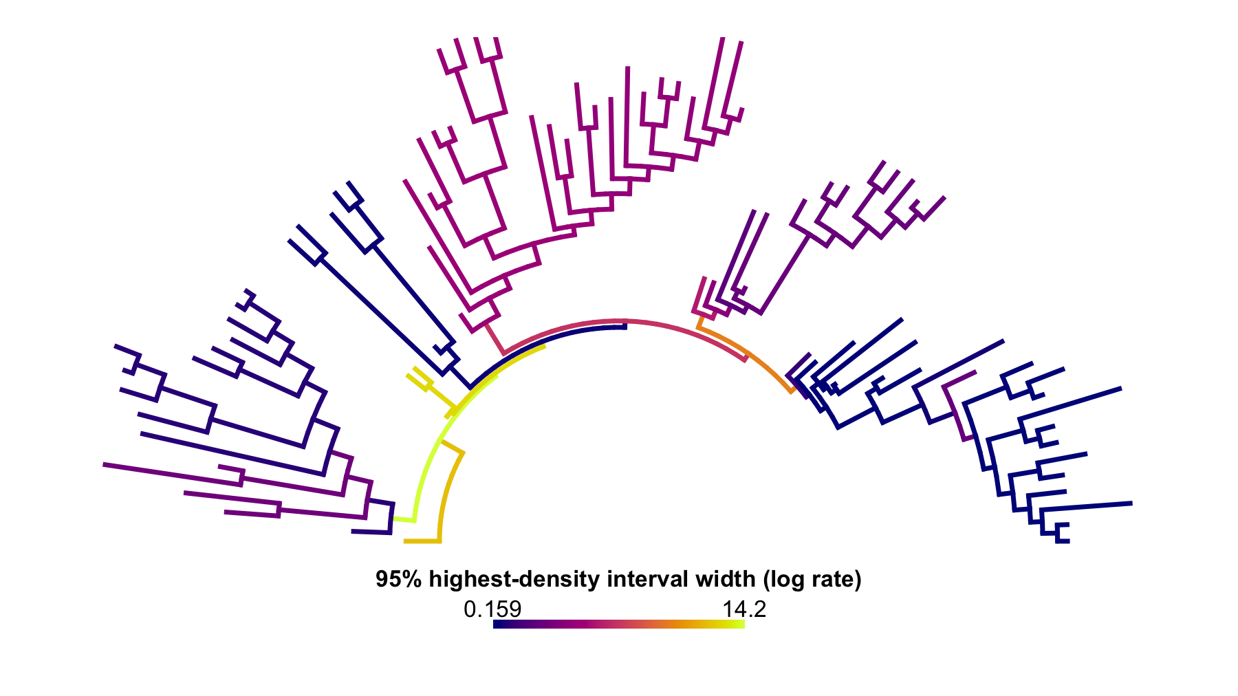
Arc-style phylogenetic tree with branches colored by the width of the across-threshold highest-density interval in fitted log-rate.

Figure 3. Across-threshold 95% shortest-interval width. This uncertainty map recolors the equal-weight rateMap() object by the width of the highest-density, or shortest weighted, interval containing 95% of the run-level log-rate values for each branch. Wider intervals indicate less stable fitted rate assignments across threshold searches; narrower intervals indicate stronger agreement among runs.

In this example dataset, the strongest uncertainty signal partly overlaps the near-zero diagnostic. A compact way to check that overlap is to mark branches in the upper quartile of highest_density_interval_width, then ask whether near-zero branches are overrepresented in that high-uncertainty set.

rate_intervals <- jaw_rate_map_equal$intervals
near_zero <- rate_intervals$is_near_zero %in% TRUE
high_interval_width <- rate_intervals$highest_density_interval_width >=
  quantile(rate_intervals$highest_density_interval_width, 0.75, na.rm = TRUE)

branch_set_n <- c(
  nrow(rate_intervals),
  sum(high_interval_width)
)
near_zero_n <- c(
  sum(near_zero),
  sum(near_zero & high_interval_width)
)

uncertainty_overlap_summary <- data.frame(
  branch_set = c(
    "all branches",
    "high-uncertainty branches"
  ),
  branches = branch_set_n,
  near_zero_branches = near_zero_n,
  near_zero_percent = sprintf("%.1f%%", 100 * near_zero_n / branch_set_n)
)
uncertainty_overlap_summary

branch_set	branches	near_zero_branches	near_zero_percent
all branches	170	54	31.8%
high-uncertainty branches	44	34	77.3%

Table 3. Near-zero enrichment among high-uncertainty branches. High-uncertainty branches are branches in the upper quartile of highest_density_interval_width. The near-zero fraction is higher in that set than across all branches.

In this sweep, near-zero branches are enriched among high-uncertainty branches: 31.8% of all branches are near-zero, compared with 77.3% in the upper quartile of shortest-interval width. This overlap is diagnostic, not redundant: near-zero flags summarize mean fitted branch rate, while uncertainty columns summarize across-threshold variation. Regular branches can still be high-uncertainty when their rates move toward or away from the lower tail.

High mean log-rate with low across-threshold uncertainty is the strongest visual cue for a robust fast-rate region. High mean log-rate with high uncertainty is more fragile: it may depend on the threshold setting, or it may identify a branch whose regime assignment changes across the sweep.

The plotted summary object still stores one row per branch under the default summary = "branch"; Appendix D shows how to sort those rows for reporting.

Same-Topology Tree Samples

The same machinery can summarize fitted rates across a posterior sample of time-calibrated trees when the topology is fixed but divergence times and branch lengths vary. For example, a researcher might fit bifrost to a set of posterior chronograms from a divergence-time analysis, then ask how the fitted branch-rate pattern can be summarized on one reference tree.

In that case, provide an explicit target_tree and relax the tree check from identical branch lengths to matching topology with control = list(check = "topology"). The target can be an MCC tree, a posterior mean chronogram, or another biologically preferred same-topology summary tree. Topology-varying posterior samples are outside the current rateMap() workflow; supporting that case would require a future extension that can summarize clades absent from some sampled trees.

For ordinary bifrost outputs, shifts are placed at nodes, so each branch has one fitted regime-rate value. With the default summary = "branch", rateMap() matches each target-tree branch to the corresponding input-tree branch by descendant tip set. The matched input branch contributes its fitted regime rate for that run, and those branch-level values are averaged across runs using the requested weighting scheme. The target tree supplies the reference topology, edge order, branch lengths, and plotting geometry for the final map. Use summary = "interval" only for true stochastic-map inputs where states can change within branches.

For posterior tree samples, weights = "equal" is usually the appropriate choice: each retained tree is one posterior draw, so the goal is to average over uncertainty in the underlying tree geometry rather than to weight alternative threshold or parameter-sweep outcomes by IC support. Keep uncertainty = TRUE to record how much the matched branch rates vary across the tree sample.

The chunk below is a template for same-topology posterior tree samples. Because this worked example uses the same jaw-shape tree as the target, it does not show a separate plot.

# Replace this with an MCC tree, posterior mean chronogram, or other
# same-topology reference tree when analyzing posterior tree samples.
jaw_target_tree <- fish.tree

jaw_target_rate_map <- rateMap(
  jaw_threshold_runs,
  target_tree = jaw_target_tree,
  weights = "equal",
  summary = "branch",
  uncertainty = TRUE,
  progress = TRUE,
  control = list(check = "topology")
)

Practical Takeaways

Holding min_descendant_tips = 10 fixed keeps the candidate-node filter constant while shift_acceptance_threshold changes.
Equal weights summarize robustness across selected threshold settings; IC weights emphasize lower-IC threshold outcomes.
For same-topology posterior tree samples with different branch lengths, use an explicit target tree, control = list(check = "topology"), branch summaries, and equal weights.
The default branch-level, log-rate-category map matches bifrost’s node-shift model.
In plot(x, ...), n_categories sets the target number of automatic category bins; category_bin_method = "equal" and category_breaks give more direct bin control; ncolors controls continuous ramps.
Uncertainty maps identify branches where inferred log-rates are stable or threshold-sensitive.

Conclusion

The single-run jaw-shape analysis identifies one supported multi-regime configuration, but it is not the only useful view of the empirical signal. A threshold sweep keeps the biological sampling constraint fixed and asks whether the inferred rate pattern survives more permissive or more conservative shift acceptance. rateMap() turns that sweep into maps and tables that separate robust high-rate regions from threshold-sensitive ones. In this jaw-shape sweep, the highest log-rate lungfish-rich region remains stable across equal-weight and IC-weighted summaries, while several moderate-rate branches are more sensitive to threshold and weighting choices.

This empirical sensitivity analysis complements simulation-based model performance assessment. Simulations show how the method behaves when the truth is known; rate maps show how one dataset behaves across plausible analysis choices.

Appendix

A. Full IC Category Metadata

The main IC-weighted category table above is intentionally condensed so it can be read next to the figure it explains. The full generated table, including color_bin, lower, upper, color, value_min, and value_max, is written with the vignette artifacts as rate_map_ic_categories.csv for readers who need the complete display metadata.

B. Original-Scale Rates

The default log-rate scale is often the easier scale for comparing multiplicative differences in fitted rates. Use log = FALSE when you need the original fitted-rate units. Print or plot the resulting object the same way as the log-rate maps above. The generated summary table below keeps the rendered preview concrete: these original-scale fitted-rate summaries remain strictly positive, and values below one correspond to negative values on the default log-rate maps.

jaw_raw_rate_map <- rateMap(
  jaw_threshold_runs,
  weights = "equal",
  uncertainty = TRUE,
  log = FALSE,
  progress = TRUE
)
plot(
  jaw_raw_rate_map,
  palette = "Viridis",
  legend_title = "Mean fitted rate"
)

quantity	value
branches	170
minimum mean fitted rate	8.07 x 10^-10
median mean fitted rate	1.90 x 10^-7
maximum mean fitted rate	1.11 x 10^-5
branches with mean fitted rate below 1	170

Table 4. Original-scale branch-rate summary. Concise generated summary of the equal-weight log = FALSE branch map. All rows summarize the plotted arithmetic mean fitted rates on the original rate scale; the below-one count explains why the default log-rate summaries can be negative without implying invalid fitted rates.

C. Continuous Interval Maps

The branch-category default is the closest match for ordinary bifrost output, because fitted bifrost shifts occur at nodes. The package stores these results using stochastic-map infrastructure, but the fitted map is not a simulated stochastic history with additional state changes inside branches. For that reason, the main summaries above use summary = "branch".

rateMap() can also use summary = "interval" for inputs that really do change state within branches, such as stochastic maps whose states can be mapped to numerical rates. In that setting, interval mode slices each target-tree branch on a shared depth grid and projects the stochastic-map segments onto those intervals. That is useful for true within-branch histories, but it is less informative for the jaw-shape bifrost sweep, where the interval map would mostly restate the branch-level result with a different plotting convention.

D. Branch Summary Table

For reporting, sort branches by their central log-rate estimate and carry along the uncertainty columns. The rendered table translates the top rows into descendant-tip counts and representative taxa. In this run, the highest log-rate whole-branch summaries point to the same lungfish-rich region highlighted above.

branch_rates <- jaw_rate_map_equal$intervals
highest_log_rate_branches <- branch_rates[
  order(branch_rates$value, decreasing = TRUE),
  c(
    "edge", "parent", "child", "clade_key",
    "value", "mean", "median", "sd",
    "q025", "q975", "highest_density_interval_low", "highest_density_interval_high", "n"
  )
]
highest_log_rate_branches$clade_key <- vapply(
  highest_log_rate_branches$clade_key,
  rate_map_format_clade_key,
  character(1)
)

head(highest_log_rate_branches, 10)

edge	tips	example_taxa	value	sd	hdi_width
13	9	Griphognathus sculpta; Griphognathus whitei; …	-11.41	0.06431	0.1786
14	6	Griphognathus sculpta; Griphognathus whitei; …	-11.41	0.06431	0.1786
15	4	Griphognathus sculpta; Griphognathus whitei; …	-11.41	0.06431	0.1786
16	3	Griphognathus sculpta; Griphognathus whitei; …	-11.41	0.06431	0.1786
17	2	Griphognathus sculpta; Griphognathus whitei	-11.41	0.06431	0.1786
18	1	Griphognathus sculpta	-11.41	0.06431	0.1786
19	1	Griphognathus whitei	-11.41	0.06431	0.1786
20	1	Rhynchodipterus elginensis	-11.41	0.06431	0.1786
21	1	Robinsondipterus longi	-11.41	0.06431	0.1786
23	1	Holodipterus gogoensis	-11.41	0.06431	0.1786

Table 5. Highest log-rate branches. Rows shown are the highest branch-level summaries after sorting by the equal-weight mean fitted log-rate. tips gives the descendant-tip count, example_taxa lists representative descendants, and hdi_width is the default 95% shortest-interval width. Repeated values reflect a single high-rate region whose descendant branches share very similar fitted rate histories across the threshold sweep.

E. Weighting-Scheme Diagnostic

The main comparison between weighting schemes is visual: compare the equal-weight map from Part 1 with the IC-weighted map in Figure 1. This appendix section gives the code and table for a more mechanical diagnostic: compare equal-weight and IC-weighted branch summaries directly to find branches where the better-supported threshold outcomes emphasize different log-rates than the unweighted sensitivity average.

equal_branch_map <- rateMap(
  jaw_threshold_runs,
  summary = "branch",
  weights = "equal",
  progress = TRUE
)

ic_branch_map <- rateMap(
  jaw_threshold_runs,
  summary = "branch",
  weights = "ic",
  progress = TRUE
)

comparison <- merge(
  equal_branch_map$intervals[, c("edge", "value")],
  ic_branch_map$intervals[, c("edge", "value")],
  by = "edge",
  suffixes = c("_equal", "_ic")
)
comparison$difference <- comparison$value_ic - comparison$value_equal
comparison$abs_difference <- abs(comparison$difference)
comparison <- comparison[order(comparison$abs_difference, decreasing = TRUE), ]

head(comparison, 10)

edge	tips	example_taxa	equal	ic	difference	abs_diff
2	69	Achoania jarvikii; Arquatichthys porosus; …	-22.3	-25.79	-3.488	3.488
139	16	Austelliscus ferox; Cheirolepis jonesi; …	-22.3	-25.79	-3.488	3.488
1	85	Achoania jarvikii; Arquatichthys porosus; …	-24.2	-25.79	-1.589	1.589
170	1	Megamastax amblyodus	-24.2	-25.79	-1.589	1.589
3	66	Arquatichthys porosus; Asperocephalus milleri; …	-16.65	-15.06	1.586	1.586
134	3	Achoania jarvikii; Guiyu oneiros; …	-16.65	-15.06	1.586	1.586
135	2	Achoania jarvikii; Psarolepis romeri	-16.65	-15.06	1.586	1.586
136	1	Achoania jarvikii	-16.65	-15.06	1.586	1.586
137	1	Psarolepis romeri	-16.65	-15.06	1.586	1.586
138	1	Guiyu oneiros	-16.65	-15.06	1.586	1.586

Table 6. Equal-weight and IC-weighted branch differences. Rows shown have the largest absolute differences between equal-weight and IC-weighted mean log-rate summaries. tips and example_taxa summarize the descendant clade; equal and ic are the two mean log-rate summaries; difference is ic - equal; and abs_diff is the absolute magnitude of that change.

Small differences suggest the broad branch log-rate picture is not very sensitive to weighting choice. Large differences deserve closer inspection, especially on branches central to the biological interpretation. Here the largest differences occur on a few moderate-rate clades and singleton branches; the highest log-rate lungfish-rich branches remain high under both weighting schemes.

Acknowledgements and Provenance

The rateMap() plotting layer follows the phytools SIMMAP plotting ecosystem described in Part 1: rate-valued summaries are drawn using the same lineage of tools as densityMap(), plotSimmap(), and plotTree().

This vignette was developed with assistance from OpenAI tools for drafting and editing; all scientific content, interpretation, and final decisions were reviewed by the authors.

References

Clavel, J., Aristide, L., and Morlon, H. (2019). A Penalized Likelihood Framework for High-Dimensional Phylogenetic Comparative Methods and an Application to New-World Monkeys Brain Evolution. https://doi.org/10.1093/sysbio/syy045
Otsu, N. (1979). A threshold selection method from gray-level histograms. IEEE Transactions on Systems, Man, and Cybernetics, 9(1), 62-66. https://doi.org/10.1109/TSMC.1979.4310076
Paradis, E., and Schliep, K. (2019). ape 5.0: an environment for modern phylogenetics and evolutionary analyses in R. Bioinformatics, 35, 526-528. https://doi.org/10.1093/bioinformatics/bty633
Revell, L. J. (2013). Two new graphical methods for mapping trait evolution on phylogenies. Methods in Ecology and Evolution, 4, 754-759.
Revell, L. J. (2014). Graphical methods for visualizing comparative data on phylogenies. Chapter 4 in Modern Phylogenetic Comparative Methods and Their Application in Evolutionary Biology: Concepts and Practice, 77-103.
Revell, L. J. (2024). phytools 2.0: an updated R ecosystem for phylogenetic comparative methods (and other things). PeerJ, 12, e16505. https://doi.org/10.7717/peerj.16505
Troyer, E. M., et al. (2025). Macroevolutionary role reversals in the earliest radiation of bony fishes. https://doi.org/10.1016/j.cub.2025.08.008

Software Used in This Vignette

bifrost for shift searches and rateMap() summaries.
ape and phytools for phylogenetic data structures, SIMMAP trees, and plotting.