Passerine Body Plan Evolution, Part 5: Post-hoc Integration and Covariance Structure • bifrost

Introduction

Berv et al. (2026) asked a post-hoc temporal integration question: do regimes inferred as faster or slower in the scalar bifrost search also differ in independently refit covariance structure? Parts 1-4 establish the temporal shift model, lineage-rate summaries, shift timing, and shift-magnitude comparisons; Part 5 asks whether those same temporal regimes carry a covariance-structure signal.

The key modeling point is what the scalar search can and cannot test. The fitted bifrost shift model estimates scalar transformations of a shared phenotypic variance-covariance matrix. Its search$VCVs component is useful for inspecting the joint model, but because those matrices are proportional scalings of a shared covariance estimate, they cannot by themselves show whether regimes have reconfigured trait integration. The workflow below makes that question explicit: it refits independent Brownian-motion mvgls() models within contemporary mapped regimes, extracts separate post-hoc covariance matrices, and summarizes their variance and correlation structure.

Berv et al. (2026) used this temporal post-hoc integration workflow for Supplementary Text 2.1 and Supplementary Figure 4. The paper also includes spatial/local assemblage covariance analyses, but those use a separate data structure and are not folded into this vignette.

This vignette has two goals. First, it shows how the Berv et al. (2026) post-hoc workflow maps onto reusable bifrost functions for fitting, summarizing, plotting, pGLS, PCA, and module diagnostics. Second, it recomputes the reported Supplementary Text 2.1 and Supplementary Figure 4 summaries from compact post-hoc artifacts, without shipping the full archived model object.

The analysis unfolds in three checks: global rate-variance and rate-integration relationships across sensitivity runs, a representative collapsed-regime pGLS, and a focal PCA of post-hoc correlation structure with module diagnostics.

Inputs and analysis settings

The full analysis object, runs_with_posthoc.rds in the Berv et al. (2026) Zenodo archive, stores complete mvgls fits and is too large for a package vignette. The package instead ships compact artifacts: all-run variance/correlation summaries, representative pGLS anchors, focal min10.ic20.gic post-hoc correlation matrices after the stricter tip-count filter used for Supplementary Figure 4, PCA inputs, trait labels, module definitions, and provenance.

# Resolve the package-local compact inputs used throughout this part.
trait_path <- system.file(
  "extdata",
  "avian-skeleton",
  "passerine_bodyplan_data.RDS",
  package = "bifrost"
)
posthoc_path <- system.file(
  "extdata",
  "avian-skeleton",
  "passerine_bodyplan_posthoc_integration_compact.RDS",
  package = "bifrost"
)
sensitivity_path <- system.file(
  "extdata",
  "avian-skeleton",
  "passerine_bodyplan_search_sensitivity_compact.RDS",
  package = "bifrost"
)
stopifnot(nzchar(trait_path), nzchar(posthoc_path), nzchar(sensitivity_path))

# Load the species-level matrix, compact sensitivity searches, and post-hoc bundle.
bodyplan_traits <- readRDS(trait_path)
bodyplan_sensitivity_searches <- readRDS(sensitivity_path)
posthoc_bundle <- readRDS(posthoc_path)

# Check what the compact post-hoc object keeps for vignette-scale checks.
data.frame(
  summary_runs = length(posthoc_bundle$vars_cors),
  focal_posthoc_matrices = length(posthoc_bundle$correlation_matrices),
  matrix_traits = nrow(posthoc_bundle$correlation_matrices[[1]]),
  compact_size_mb = round(file.info(posthoc_path)$size / 1024^2, 3)
)
#>   summary_runs focal_posthoc_matrices matrix_traits compact_size_mb
#> 1           12                     58            12           0.129

The minimum-tip thresholds serve two different parts of the workflow. Independent covariance refits need enough contemporary tips to estimate a regime matrix at all, so fit_regime_covariances() attempts a refit when a regime has at least posthoc_fit_min_tips tips (>=). The PCA is more sensitive to small, noisy matrices, so regime_correlation_pca() uses a stricter filter, retaining only regimes with tip_count > pca_min_tips (>). These values reproduce the Supplementary Figure 4 analysis in Berv et al. (2026), while keeping the thresholds visible for other datasets.

# Read the archived analysis settings from the compact bundle.
posthoc_fit_min_tips <- posthoc_bundle$settings$fit_min_tips
pca_min_tips <- posthoc_bundle$settings$pca_min_tips
remove_high_corr <- posthoc_bundle$settings$remove_high_corr
posthoc_corr_threshold <- posthoc_bundle$settings$corr_threshold

# Keep filtering and plotting choices visible so users can tune them.
resid_sd_threshold_vars <- 2
resid_sd_threshold_corrs <- 2
plot_bootstrap_reps <- 250
plot_ci_level <- 0.99

# Report the settings that control the reproducibility checks in this vignette.
data.frame(
  posthoc_fit_min_tips = posthoc_fit_min_tips,
  pca_min_tips = pca_min_tips,
  pca_tip_filter = posthoc_bundle$settings$pca_tip_filter,
  remove_high_corr = remove_high_corr,
  corr_threshold = posthoc_corr_threshold,
  residual_sd_threshold = resid_sd_threshold_vars,
  bootstrap_reps = plot_bootstrap_reps,
  plot_ci_level = plot_ci_level
)
#>   posthoc_fit_min_tips pca_min_tips           pca_tip_filter remove_high_corr
#> 1                    2           10 tip_count > pca_min_tips             TRUE
#>   corr_threshold residual_sd_threshold bootstrap_reps plot_ci_level
#> 1           0.95                     2            250          0.99

Generic API workflow

The compact object avoids rerunning all archived refits during vignette builds. For a new dataset, the public API follows the same post-hoc sequence: start from a named list of bifrost_search objects, refit independent models on valid contemporary regime subtrees, summarize those fits by named regime IDs, and run the rate-integration and PCA summaries from the resulting tables. The plural wrappers handle named sensitivity runs; cores controls parallel fitting of regime subtrees within each run.

# Refit independent BM covariance models for every sensitivity run.
posthoc_fits_by_run <- fit_regime_covariance_runs(
  bodyplan_sensitivity_searches,
  trait_data = bodyplan_traits,
  formula = trait_data[, c(-13)] ~ trait_data[, c(13)],
  model = "BM",
  min_tips = posthoc_fit_min_tips,
  cores = 8,
  error = TRUE
)

# Convert each fitted-regime object into variance/correlation summaries.
posthoc_summaries <- summarize_regime_covariance_runs(
  posthoc_fits_by_run,
  searches = bodyplan_sensitivity_searches,
  remove_high_corr = remove_high_corr,
  corr_threshold = posthoc_corr_threshold
)

# Pool the sensitivity runs for the global Supplementary Figure 4A relationships.
supp4a_relationships <- regime_integration_relationships(
  posthoc_summaries,
  resid_sd_threshold_vars = resid_sd_threshold_vars,
  resid_sd_threshold_corrs = resid_sd_threshold_corrs,
  n_boot = plot_bootstrap_reps,
  ci_level = plot_ci_level
)

# Fit the representative collapsed-regime pGLS reported in Supplementary Text 2.1.
representative_pgls <- regime_integration_pgls(
  posthoc_summaries$min20.ic20.gic,
  search = bodyplan_sensitivity_searches$min20.ic20.gic
)

# Run the focal PCA on post-hoc correlation matrices after the strict tip filter.
focal_pca <- regime_correlation_pca(
  posthoc_fits_by_run$min10.ic20.gic,
  min_tips = pca_min_tips,
  trait_labels = posthoc_bundle$trait_labels
)

# Score biologically named trait modules against the focal PCA axes.
focal_modules <- regime_module_diagnostics(
  focal_pca,
  modules = posthoc_bundle$modules,
  comparisons = list(
    within_wing = c("wing_flight", "wing_flight"),
    hindcran_wing = c("hindlimb_cranial", "wing_flight"),
    cranial_hindlimb = c("cranial", "hindlimb"),
    cranial_wing = c("cranial", "wing_flight")
  ),
  pcs = 1:4
)

The important guardrail is that each object returned by fit_regime_covariances() contains independent post-hoc regime covariances. Those matrices, and the compact posthoc_bundle$correlation_matrices, are not the proportional VCVs stored on a scalar bifrost_search result.

Global rate and integration summaries

Do faster temporal regimes also show higher variance or altered integration? Following Berv et al. (2026), this is an interpretation check rather than an additional search model. The scalar BMM search finds regimes that differ in overall evolutionary rate; the post-hoc refits ask whether those same mapped regimes also have independently estimated covariance matrices with larger average variance or weaker average trait correlations. Biologically, weaker global integration is the pattern expected when skeletal traits are less tightly constrained to vary together and can evolve more independently.

To ask that question, Berv et al. summarized each post-hoc regime covariance matrix by its mean variance and mean absolute trait correlation. The plots below pool the 12 sensitivity runs used for Supplementary Figure 4A. They show the two global relationships: jointly inferred regime rates are positively associated with post-hoc variance and negatively associated with post-hoc integration.

# Use the compact all-run variance/correlation summaries.
vars_cors <- posthoc_bundle$vars_cors

# Rebuild the global rate-integration object with the Supplementary Figure 4A filters.
supp4a_relationships <- regime_integration_relationships(
  vars_cors,
  resid_sd_threshold_vars = resid_sd_threshold_vars,
  resid_sd_threshold_corrs = resid_sd_threshold_corrs,
  n_boot = plot_bootstrap_reps,
  ci_level = plot_ci_level,
  seed = 1
)

# Extract fitted slopes and point counts for a compact numerical check.
supp4a_models <- as.data.frame(supp4a_relationships, component = "models")
data.frame(
  regimes = nrow(as.data.frame(supp4a_relationships, component = "combined")),
  runs = length(unique(supp4a_relationships$combined$run)),
  variance_points_after_filter = nrow(as.data.frame(supp4a_relationships, component = "variance_points")),
  correlation_points_after_filter = nrow(as.data.frame(supp4a_relationships, component = "correlation_points")),
  variance_slope = supp4a_models$slope[supp4a_models$panel == "variance"],
  correlation_slope = supp4a_models$slope[supp4a_models$panel == "correlation"]
)
#>   regimes runs variance_points_after_filter correlation_points_after_filter
#> 1     362   12                          346                             338
#>   variance_slope correlation_slope
#> 1      0.9240046         -2.905217

# Use the S3 plot method to draw the variance and correlation panels together.
plot(
  supp4a_relationships,
  panel = "both"
)

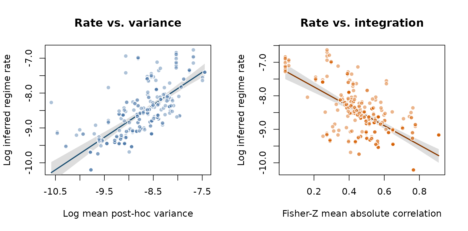
Figure 1. Global post-hoc regime rate-integration relationships. Each panel pools independently refit regime covariance summaries across the 12 temporal sensitivity runs. After the residual filters used for Supplementary Figure 4A, faster fitted BMM regimes have higher mean variance and lower mean absolute trait correlation.

Representative pGLS result

The representative pGLS model in Supplementary Text 2.1 used min20.ic20.gic. regime_integration_pgls() reproduces that check by collapsing the mapped tree to monophyletic regime tips, scaling the post-hoc summary variables as in the original formula, and fitting phylolm(model = "BM").

# Refit the representative pGLS from the compact post-hoc summary table.
pgls_fit <- regime_integration_pgls(
  posthoc_bundle$vars_cors$min20.ic20.gic,
  search = bodyplan_sensitivity_searches$min20.ic20.gic
)
#> Warning: The pGLS collapse dropped nonmonophyletic regime(s): 186, 42, 46, 12,
#> 17, 62, 106, 41, 4, 16, 52. All tips assigned to these regimes were removed,
#> matching the manuscript workflow.

# Put estimates and standard errors into a small readable coefficient table.
pgls_coef <- data.frame(
  term = names(pgls_fit$coefficients),
  estimate = unname(pgls_fit$coefficients),
  std_error = sqrt(diag(pgls_fit$vcov)),
  row.names = NULL,
  check.names = FALSE
)
pgls_coef$estimate <- round(pgls_coef$estimate, 3)
pgls_coef$std_error <- round(pgls_coef$std_error, 3)

# Report the published anchor values without printing the full model object.
list(
  r_squared = round(pgls_fit$r.squared, 3),
  df_residual = pgls_fit$n - length(pgls_fit$coefficients),
  coefficients = pgls_coef
)
#> $r_squared
#> [1] 0.841
#> 
#> $df_residual
#> [1] 25
#> 
#> $coefficients
#>                               term estimate std_error
#> 1                      (Intercept)   -0.122     0.212
#> 2                 scale(log(vars))    0.538     0.065
#> 3 scale(fisher_z_transform(corrs))   -0.491     0.062

The key standardized effects match the supplement: scale(log(vars)) is approximately 0.54, scale(fisher_z_transform(corrs)) is approximately -0.49, and the model explains about 84% of the variance in the representative collapsed-regime pGLS. Together with Figure 1, this recapitulates the Berv et al. (2026) conclusion that the temporal rate signal is associated with both greater independently estimated variance and reduced global phenotypic integration, not only a proportional rescaling of one covariance matrix.

Correlation-structure PCA

The focal PCA uses the min10.ic20.gic post-hoc regime correlation matrices after keeping regimes with more than 10 tips. regime_correlation_pca() is generic: it accepts any named list of same-dimension covariance or correlation matrices, vectorizes the upper triangle, and returns scores, loadings, variance explained, and diagnostics as ordinary data frames.

# Vectorize same-dimension post-hoc correlation matrices and run PCA.
posthoc_pca <- regime_correlation_pca(
  posthoc_bundle$correlation_matrices,
  tip_counts = posthoc_bundle$pca_inputs$tip_counts,
  regime_ages = posthoc_bundle$pca_inputs$regime_ages,
  trait_labels = posthoc_bundle$trait_labels,
  min_tips = pca_min_tips
)

# Convert S3 components to data frames for inspection or downstream plotting.
pca_variance <- as.data.frame(posthoc_pca, component = "variance")
pca_scores <- as.data.frame(posthoc_pca, component = "scores")
pca_loadings <- as.data.frame(posthoc_pca, component = "loadings")

# Preview the first four axes and their cumulative explanatory power.
pca_variance[1:4, c("PC", "variance_explained", "cumulative_variance")]
#>    PC variance_explained cumulative_variance
#> 1 PC1         0.39890908           0.3989091
#> 2 PC2         0.11960598           0.5185151
#> 3 PC3         0.07127841           0.5897935
#> 4 PC4         0.06523424           0.6550277

PC1-PC4 explain 39.89%, 11.96%, 7.13%, 6.52% of the focal correlation-structure variation. Figure 2 uses the clustered loading view from Supplementary Figure 4: each PC is reclustered locally so the strongest positive and negative trait-pair blocks are easier to read. Each off-diagonal cell is a PCA loading for one pairwise trait correlation, not an observed correlation in a single regime. Positive and negative colors mark trait pairs that contribute in opposite directions along the same correlation-structure axis. When ComplexHeatmap is installed, plot() uses that renderer; otherwise it falls back to clustered base graphics.

Berv et al. (2026) interpret PC1 as the dominant covariance-structure axis: it separates a distal wing/flight module from hindlimb and cranial traits. PC2-PC4 add subtler structure involving cranial-to-hindlimb coupling, distal autopod correlations, and the keel/furcula as pectoral elements that link multiple skeletal regions. The heatmaps are therefore most useful as a map of which trait-pair correlations move together across regimes, while the module diagnostics below make the main biological contrasts explicit.

# Reconstruct each PC loading vector as a trait-by-trait heatmap.
plot(
  posthoc_pca,
  type = "loadings",
  components = 1:4,
  cluster = "local",
  heatmap_engine = "auto",
  show_dendrogram = TRUE,
  show_legend = TRUE,
  # Label each panel with the variance explained by that PCA axis.
  main = paste0(
    "PC",
    1:4,
    " loadings (",
    round(100 * posthoc_pca$variance_explained[1:4], 1),
    "%)"
  )
)

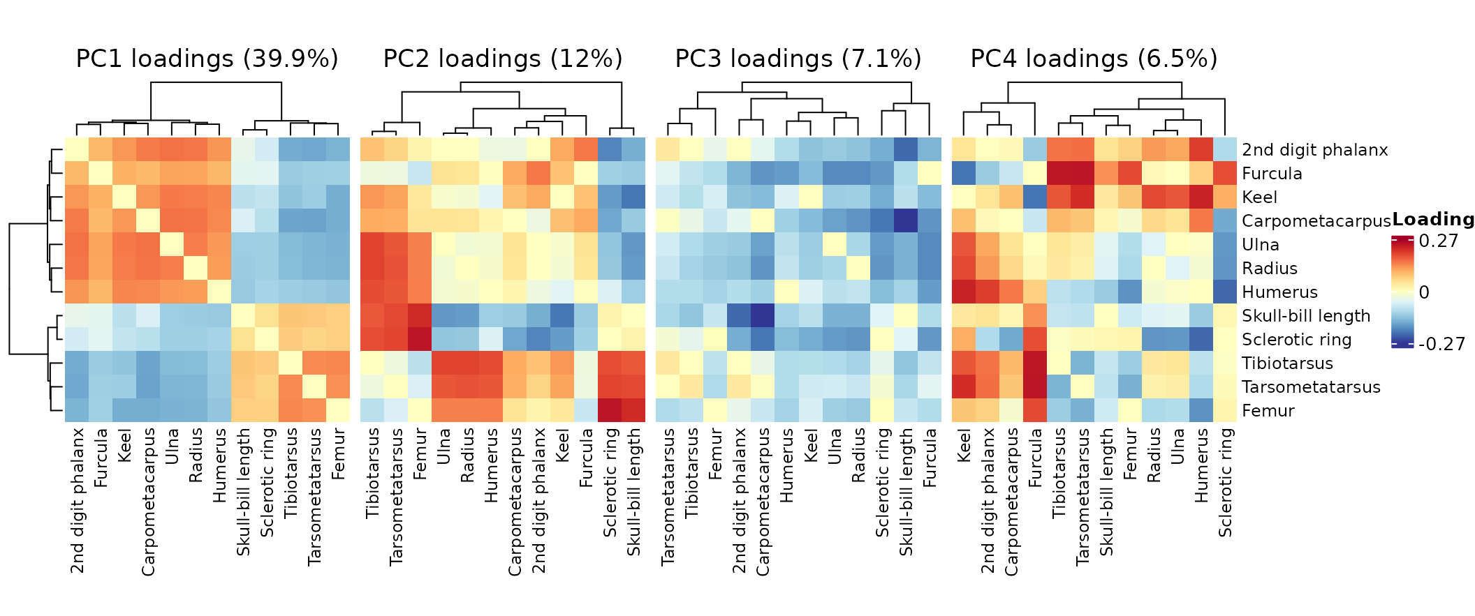
Figure 2. Focal post-hoc correlation PCA loadings. Heatmaps reconstruct PC1-PC4 upper-triangle correlation loadings as trait-by-trait matrices for the focal min10.ic20.gic post-hoc matrices after the stricter tip-count filter. Local row and column clustering in each panel echoes the Supplementary Figure 4B-C heatmap view and highlights the trait-pair blocks that define each covariance-structure axis.

Module diagnostics

The PCA axes can be interpreted by comparing regime scores with biologically named trait modules. Here we use the module contrasts highlighted by Berv et al. (2026): wing/flight integration versus cranial and hindlimb coupling. The compact bundle stores the trait-to-module assignments, shown below before the contrasts are defined. hindlimb_cranial is a composite module used for the PC1 diagnostic, not a separate anatomical region.

# Pull the named trait modules stored with the compact post-hoc bundle.
bodyplan_modules <- posthoc_bundle$modules

# Print the trait-to-module assignments before defining pairwise contrasts.
module_assignments <- data.frame(
  module = rep(names(bodyplan_modules), lengths(bodyplan_modules)),
  trait = unlist(bodyplan_modules, use.names = FALSE),
  row.names = NULL
)
module_assignments
#>              module             trait
#> 1       wing_flight   Carpometacarpus
#> 2       wing_flight 2nd digit phalanx
#> 3       wing_flight            Radius
#> 4       wing_flight              Ulna
#> 5       wing_flight           Humerus
#> 6       wing_flight              Keel
#> 7       wing_flight           Furcula
#> 8          hindlimb       Tibiotarsus
#> 9          hindlimb   Tarsometatarsus
#> 10         hindlimb             Femur
#> 11          cranial Skull-bill length
#> 12          cranial    Sclerotic ring
#> 13 hindlimb_cranial       Tibiotarsus
#> 14 hindlimb_cranial   Tarsometatarsus
#> 15 hindlimb_cranial             Femur
#> 16 hindlimb_cranial Skull-bill length
#> 17 hindlimb_cranial    Sclerotic ring

# Define module-pair contrasts using the module names shown above.
module_comparisons <- list(
  within_wing = c("wing_flight", "wing_flight"),
  hindcran_wing = c("hindlimb_cranial", "wing_flight"),
  cranial_hindlimb = c("cranial", "hindlimb"),
  cranial_wing = c("cranial", "wing_flight")
)

# Compute per-regime module summaries, then correlate them with PCA scores.
module_diagnostics <- regime_module_diagnostics(
  posthoc_pca,
  modules = bodyplan_modules,
  comparisons = module_comparisons,
  pcs = 1:4
)

# Pull the diagnostic correlations into a table.
module_table <- as.data.frame(module_diagnostics, component = "correlations")

# Keep the four comparisons highlighted in Supplementary Figure 4D.
module_table <- module_table[
  (module_table$PC == "PC1" & module_table$module_comparison %in% c("within_wing", "hindcran_wing")) |
    (module_table$PC == "PC2" & module_table$module_comparison %in% c("cranial_hindlimb", "cranial_wing")),
  ,
  drop = FALSE
]

# Add reader-facing labels and round only for display.
module_table$diagnostic <- c(
  "PC1 vs within-wing mean",
  "PC1 vs hindlimb+cranial to wing mean",
  "PC2 vs cranial to hindlimb mean",
  "PC2 vs cranial to wing mean"
)
module_table$correlation <- round(module_table$correlation, 3)
module_table[, c("diagnostic", "correlation")]
#>                             diagnostic correlation
#> 1              PC1 vs within-wing mean       0.879
#> 2 PC1 vs hindlimb+cranial to wing mean      -0.934
#> 7      PC2 vs cranial to hindlimb mean       0.683
#> 8          PC2 vs cranial to wing mean      -0.566

The signs and magnitudes match the Supplementary Figure 4B-D diagnostics. PC1 increases as within-wing/flight correlations become stronger and decreases as the wing/flight module becomes more coupled to hindlimb plus cranial traits. PC2 captures a smaller head-coupling contrast: regimes with higher PC2 scores tend to emphasize cranial-hindlimb correlations more than cranial-wing correlations. This is the concise version of the Berv et al. (2026) interpretation that covariance differences vary mostly along a wing/flight versus hindlimb-cranial axis, with additional axes refining how the same anatomical regions are linked.

# Draw the same four module/PCA checks using the module-diagnostic plot method.
local({
  old_par <- par(
    pty = "s",
    mar = c(4.7, 4.8, 3.0, 0.8),
    oma = c(0, 0, 0.4, 0),
    mgp = c(2.45, 0.75, 0),
    las = 1
  )
  on.exit(par(old_par), add = TRUE)

  plot(
    module_diagnostics,
    pc = c("PC1", "PC1", "PC2", "PC2"),
    comparison = c(
      "within_wing",
      "hindcran_wing",
      "cranial_hindlimb",
      "cranial_wing"
    ),
    main = c(
      "PC1 vs within-wing",
      "PC1 vs hindlimb+cranial to wing",
      "PC2 vs cranial-hindlimb",
      "PC2 vs cranial-wing"
    ),
    xlab = c("PC1 score", "PC1 score", "PC2 score", "PC2 score"),
    ylab = c(
      "Within-wing corr.",
      "Hindlimb+cranial-wing corr.",
      "Cranial-hindlimb corr.",
      "Cranial-wing corr."
    ),
    point_col = c("#009E73", "#0072B2", "#CC79A7", "#D55E00"),
    line_col = c("#00664A", "#004B75", "#8A4F70", "#8A3A00"),
    ribbon_col = "grey70",
    point_alpha = 0.62,
    pch = 21,
    lwd = 2.4,
    n_boot = plot_bootstrap_reps,
    ci_level = plot_ci_level,
    seed = 3,
    cex = 1.08,
    cex.axis = 0.86,
    cex.lab = 0.92,
    cex.main = 0.98,
    bty = "l"
  )
})

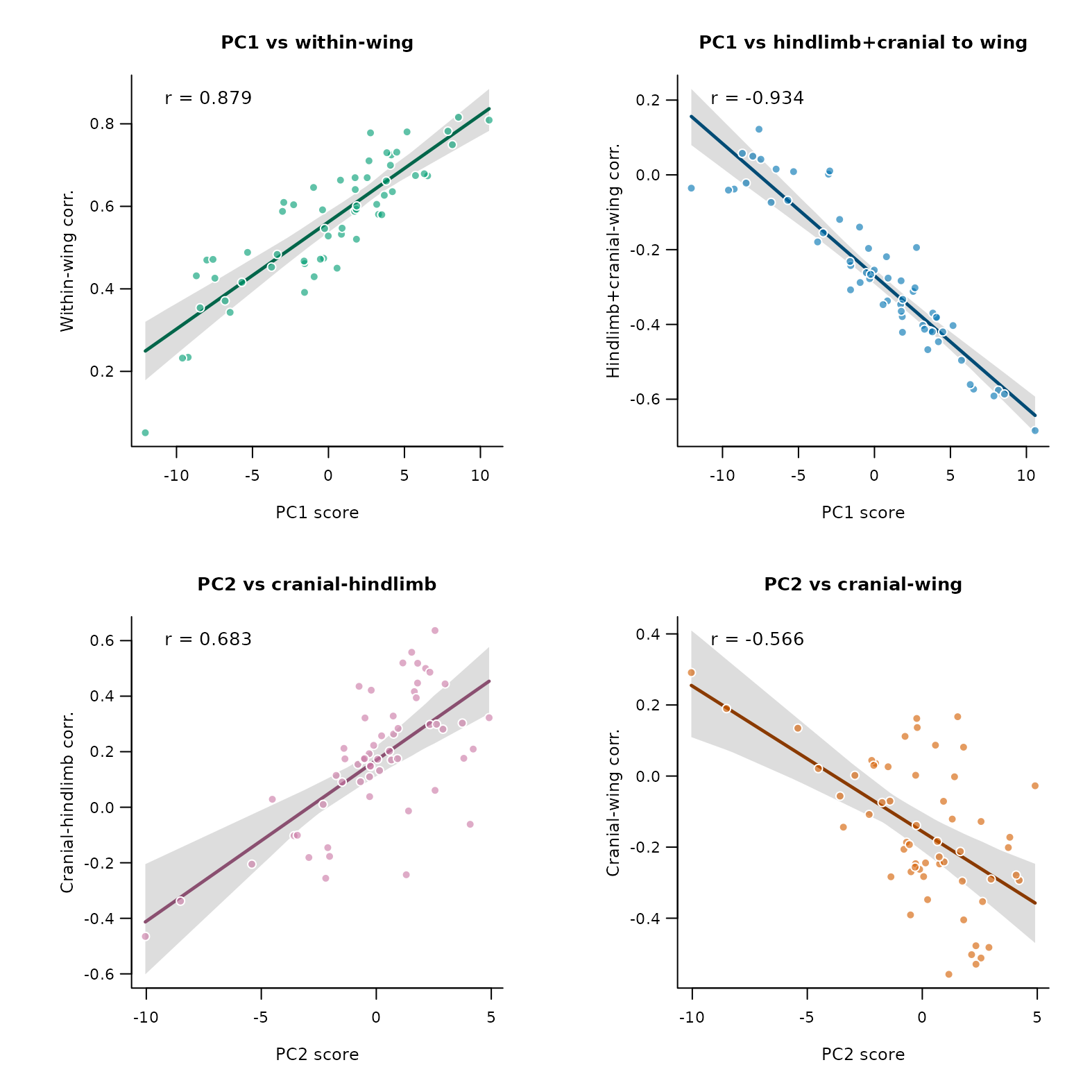
Figure 3. Module diagnostics for focal post-hoc PCA scores. Each square panel compares a PCA score with one Supplementary Figure 4D module contrast. Shaded ribbons use the same bootstrap confidence-interval settings as Figure 1. PC1 increases with within-wing/flight integration and decreases with hindlimb+cranial-to-wing coupling, while PC2 separates cranial-hindlimb from cranial-wing correlations.

Limitations

This workflow is post-hoc. It conditions on the mapped regimes selected by the scalar bifrost search, then asks whether those regimes differ in covariance structure by refitting independent within-regime models to contemporary tips. That makes it useful for testing whether inferred rate shifts align with integration changes, but it is not a joint model that estimates regime-specific covariance reconfiguration during the search.

The compact package object is not the full archived runs_with_posthoc.rds; it stores only the summaries, focal post-hoc correlation matrices, PCA inputs, labels, module definitions, and provenance needed to recompute the vignette figures and numerical checks. Use the complete Berv et al. archive when you need the full archived object graph or all fitted post-hoc model objects.

Finally, this is a temporal regime workflow. Spatial local assemblage covariance and modularity use a different data structure and should be treated in a separate spatial vignette.

Practical Takeaways

fit_regime_covariances() and fit_regime_covariance_runs() refit independent within-regime Brownian-motion covariance models after a temporal bifrost search has selected mapped regimes.
summarize_regime_covariances() and summarize_regime_covariance_runs() expose the filtering knobs used here, including remove_high_corr, corr_threshold, and named-run matching.
regime_integration_relationships() and regime_integration_pgls() summarize rate-variance and rate-correlation relationships from post-hoc matrices, not from proportional search VCVs.
regime_correlation_pca() and regime_module_diagnostics() recreate the focal Supplementary Figure 4 covariance-structure checks with generic matrix, module, and plotting methods.
Spatial/local assemblage covariance belongs in a separate workflow.

References

If you use these data or reproduce this workflow, the most relevant citations are:

Berv, Jacob S., Charlotte M. Probst, Santiago Claramunt, J. Ryan Shipley, Matt Friedman, Stephen A. Smith, David F. Fouhey, and Brian C. Weeks. 2026. “Rates of passerine body plan evolution in time and space.” Nature Ecology & Evolution. https://doi.org/10.1038/s41559-026-03110-5
Berv, Jacob S., Charlotte M. Probst, Santiago Claramunt, J. Ryan Shipley, Matt Friedman, Stephen A. Smith, David F. Fouhey, and Brian C. Weeks. 2026. “Supplementary data archive for Rates of passerine body plan evolution in time and space” (v1.0.0) [Data set]. Zenodo. https://doi.org/10.5281/zenodo.19198393
Claramunt, Santiago, Christopher Sheard, Joseph W. Brown, Guillermo Cortes-Ramirez, Joel Cracraft, Mason M. Su, Brian C. Weeks, and Joseph A. Tobias. 2025. “A new time tree of birds reveals the interplay between dispersal, geographic range size, and diversification.” Current Biology. Advance online publication. https://doi.org/10.1016/j.cub.2025.07.004
Weeks, Brian C., Zhaoqi Zhou, Charlotte M. Probst, Jacob S. Berv, Brendan O’Brien, Brett W. Benz, Hannah R. Skeen, M. Ziebell, Linde Bodt, and David F. Fouhey. 2025. “Skeletal trait measurements for thousands of bird species.” Scientific Data 12:884. https://doi.org/10.1038/s41597-025-05234-y

Software Used in This Vignette

bifrost for post-hoc regime covariance fitting, summary extraction, plotting, pGLS helpers, and PCA helpers.
mvMORPH for the underlying mvgls() refits when users run the from-scratch workflow.
phylolm for the collapsed-regime pGLS.
ape and phytools for mapped-tree and subtree operations.
future and future.apply for optional parallel regime refits.

AI Assistance

This vignette was developed with assistance from OpenAI tools for drafting, editing, and figure refinement; all scientific content, interpretation, and final decisions were reviewed by the authors.