
Passerine Body Plan Evolution, Part 2: Lineage-Rate Summaries
Source:vignettes/avian-skeleton-part-2.Rmd
avian-skeleton-part-2.RmdIntroduction
Part 2 asks how a fitted multi-regime Brownian motion model (BMM) can
be turned into a species-level summary of evolutionary tempo. The focal
bifrost search estimates scalar transformations of a
multivariate phenotypic variance-covariance matrix on a mapped
phylogeny; those fitted rates live on regimes and ancestral histories,
not directly in a tidy table of extant species.
lineage_rates() provides that bridge by collapsing each
extant species’ inherited regime history into a present-biased
lineage-rate statistic.
Berv et al. (2026) used this statistic as a way to ask whether recent evolutionary tempo inferred from deep-time rate shifts relates to contemporary species-level and assemblage-level predictors. This vignette stays at the reusable package step: it shows how the final mapped tree and fitted regime rates become one present-weighted summary per tip, while keeping the terminal fitted rate available as a separate comparison. The compact object is enough for this calculation; the full archive remains the source for proposal history, sensitivity searches, and candidate model fits.
Computing lineage-rate summaries
The purpose of lineage_rates() is to summarize the rate
history inherited by each extant lineage when the terminal regime alone
is too narrow a description. Two species can share the same terminal
fitted rate after inheriting different ancestral regimes, and two
lineages with similar recent rates can carry different amounts of deeper
history. The statistic therefore treats the mapped BMM as a
piecewise-constant history of multivariate evolutionary tempo and
computes a temporally filtered average along each root-to-tip path.
In the avian body-plan example, the state value being averaged is the
scalar BMM rate assigned to each mapped regime, interpreted by Berv et
al. (2026) as the mean of the diagonal variances in that regime’s
evolutionary variance-covariance matrix. The resulting
log_lineage_rate is not an instantaneous tip-rate estimate
or a hard recent-time-window average. It is a tunable, present-biased
summary of inherited regime history, reported by Berv et al. (2026)
under decay_base = 2, half_life = 5, and
normalized weights.
The key object is an age-decay kernel. Following the
lineage_rates() documentation, the normalized weighted
lineage-rate statistic is
\bar{r}_{\mathrm{WLR}} = \frac{1}{Z} \sum_{i=1}^{L} b^{-a_i/T} r_i
where
Z = \sum_{j=1}^{L} b^{-a_j/T}.
Here r_i is the fitted value for
ancestral node or path element i, a_i is that element’s age before the selected
reference point, b is
decay_base, T is the
half_life argument used as a decay time scale, and L is the number of included path elements.
For the top-level statistic used here, i indexes ancestral nodes along the lineage,
including the root and excluding the terminal tip state. When
half_life = NULL, the kernel is b^{-a_i} instead of b^{-a_i/T}; when
normalize_weights = FALSE, the 1/Z normalization is skipped.
The name half_life is literal only when
decay_base = 2: a path element T Myr older then receives 2^{-1} = 1/2 the raw weight of a present-day
element. More generally, an element T
Myr older receives 1/b the raw weight,
so the slider below labels T as the
decay scale while noting the manuscript half-life setting. Figure 1
shows how the settings interact, then traces those same settings through
a miniature mapped lineage before the lineage-rate table is
computed.
How decay base and decay scale shape lineage-rate memory
Decay base b = larger values concentrate weight near the present; b = 2 gives the usual half-life interpretation
Figure 1. Interactive age-decay kernels and mapped-lineage weighting. Panel A shows the selected raw age-decay kernel, with the maximum-age slider changing only that panel. Panel B converts the same kernel into normalized shares for example path elements. Panel C traces one mapped lineage through a miniature simmap tree, and the rate boxes set the regime values used by the traced lineage. Panel D applies the same decay, normalization, and rate settings; the switch toggles the 1 / Z normalization and the labels report each displayed weight, fitted rate, and collapsed estimate. The decay scale is a literal half-life only when decay_base = 2.
Loading the focal search
This part requests only the compact focal search
(passerine-search), an approximately 1.9 MB download on
first use. Later calls reuse the verified cache. This explicit command
checks for an update:
# Refresh the compact focal search only when an updated copy is wanted.
bifrost_example_file("passerine-search", refresh = TRUE)
# Load the same compact focal result inspected in Part 1.
search_path <- bifrost_example_file("passerine-search")

bodyplan_search <- readRDS(search_path)

# Preserve the S3 class if an older serialized copy lacks it.
if (!inherits(bodyplan_search, "bifrost_search")) {
  class(bodyplan_search) <- c("bifrost_search", class(bodyplan_search))
}

# Confirm that the object is a fitted BMM search with inferred shifts.
data.frame(
  inherits_bifrost_search = inherits(bodyplan_search, "bifrost_search"),
  model = bodyplan_search$model_no_uncertainty$model,
  fitted_regimes = length(bodyplan_search$model_no_uncertainty$param),
  accepted_shifts = length(bodyplan_search$shift_nodes_no_uncertainty)
)
#>   inherits_bifrost_search model fitted_regimes accepted_shifts
#> 1                    TRUE   BMM             83              82
This check confirms that the compact object is a multi-regime BMM
search, which lineage_rates() requires before computing
rate summaries from a mapped heterogeneous-rate history.
Running lineage_rates()
With the weighting scheme established and the focal search loaded,
the next step is to run the Berv et al. (2026) lineage-rate calculation.
This call uses the parameter choices described above:
decay_base = 2, half_life = 5, normalized
weights, and log-scale rates. The progress bar is suppressed so the
vignette output stays quiet.
Because each tip defines one extant lineage, the returned table has
one row per species. The preview below sorts lineages by the
inherited-history summary, log_lineage_rate, while keeping
log_tip_rate beside it. That pairing is useful because both
columns are on the log scale: the lineage summary reflects weighted
ancestral history, whereas log_tip_rate records only the
terminal fitted state.
# Run the Berv et al. (2026) lineage-rate summary.
bodyplan_lineage_rates <- lineage_rates(
  bodyplan_search,
  progress = FALSE
)

# Show the fastest lineages first and keep the most useful columns.
lineage_preview <- bodyplan_lineage_rates[
  order(bodyplan_lineage_rates$log_lineage_rate, decreasing = TRUE),
  c("tip.label", "shift_count", "log_lineage_rate", "log_tip_rate")
]
head(lineage_preview)
#>                     tip.label shift_count log_lineage_rate log_tip_rate
#> 1562   Menura_novaehollandiae           1        -4.350366    -5.856085
#> 2046    Conopophaga_ardesiaca           2        -5.749559    -5.753581
#> 2047      Conopophaga_lineata           2        -5.749559    -5.753581
#> 2003 Hylopezus_perspicillatus           2        -5.958929    -6.938088
#> 475       Rhodinocichla_rosea           6        -6.099697    -7.160269
#> 549         Fringilla_coelebs           5        -6.248063    -6.787524
To see how the temporal weighting changes this comparison, recompute the lineage summary with a much shorter half-life:
# Emphasize recent branches by recomputing lineage rates with a shorter half-life.
bodyplan_lineage_rates_short_decay <- lineage_rates(
  bodyplan_search,
  half_life = 0.5,
  progress = FALSE
)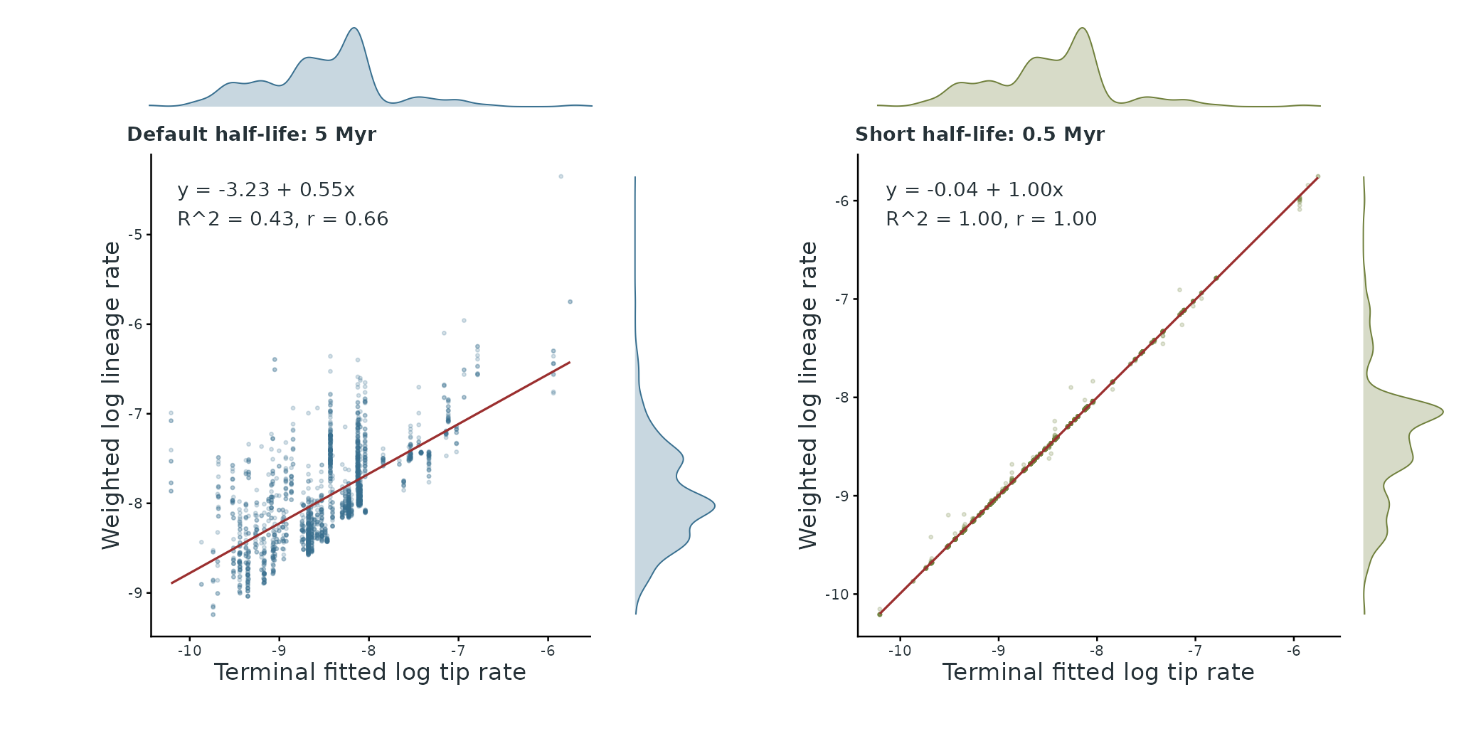
Figure 2. Decay strength controls how closely weighted lineage rates track terminal fitted log tip rates. Left: the 5 Myr half-life used by Berv et al. (2026) retains more root-to-tip history. Right: a short 0.5 Myr half-life heavily emphasizes recent branches, so the weighted lineage summary nearly collapses onto the terminal log tip-rate summary.
You can merge the resulting species-level table with ecological, geographic, or climatic metadata when asking how lineage-level inferred rates relate to external predictors. Because these summaries are still estimated for species that share ancestry, phylogenetic methods such as PGLS may remain appropriate even though the estimator concentrates signal toward the present.
Practical Takeaways
-
lineage_rates()returns one inherited BMM rate-history summary per extant root-to-tip lineage. - The Berv et al. (2026) lineage-rate statistic uses
decay_base = 2,half_life = 5, normalized weights, and log-scale fitted rates. - The age-decay kernel controls how strongly deeper ancestral history contributes to each lineage summary; shorter half-lives make the summary converge toward the terminal fitted rate.
-
log_tip_rateis intentionally separate fromlog_lineage_rate: it records only the terminal fitted state on the same log scale. - The lineage-rate table can be joined to species-level ecological, geographic, climatic, or trait metadata for downstream predictor analyses.
- Present-biased lineage-rate summaries do not remove phylogenetic non-independence; downstream models should still account for shared ancestry when the question calls for species-level inference.
- Continue to Part 3 for shift-transition tables, branch-rate annotations, fitted rate distributions, and waiting-time distributions.
References
If you use these data or reproduce this workflow, the most relevant citations are:
- Berv, Jacob S., Charlotte M. Probst, Santiago Claramunt, J. Ryan Shipley, Matt Friedman, Stephen A. Smith, David F. Fouhey, and Brian C. Weeks. 2026. “Rates of passerine body plan evolution in time and space.” Nature Ecology & Evolution. https://doi.org/10.1038/s41559-026-03110-5
- Berv, Jacob S., Charlotte M. Probst, Santiago Claramunt, J. Ryan Shipley, Matt Friedman, Stephen A. Smith, David F. Fouhey, and Brian C. Weeks. 2026. “Supplementary data archive for Rates of passerine body plan evolution in time and space” (v1.0.0) [Data set]. Zenodo. https://doi.org/10.5281/zenodo.19198393
- Claramunt, Santiago, Christopher Sheard, Joseph W. Brown, Guillermo Cortes-Ramirez, Joel Cracraft, Mason M. Su, Brian C. Weeks, and Joseph A. Tobias. 2025. “A new time tree of birds reveals the interplay between dispersal, geographic range size, and diversification.” Current Biology. Advance online publication. https://doi.org/10.1016/j.cub.2025.07.004
Software Used in This Vignette
-
bifrostfor weighted lineage-rate summaries from fitted BMM searches. -
apeandphytoolsunderlie the mapped-tree calculations used bylineage_rates(). -
ggplot2andpatchworkdraw the age-decay and lineage-rate comparison figures.