
Passerine Body Plan Evolution, Part 3: Shift Timing and Distribution Fits
Source:vignettes/avian-skeleton-part-3.Rmd
avian-skeleton-part-3.RmdIntroduction
Accepted shifts become interpretable once they are turned into explicit events: where did the regime change occur, did it increase or decrease the fitted BMM rate, how are fitted regime rates distributed, and how much time separates successive shifts? Part 3 answers those timing and distribution questions from the compact focal passerine body-plan search.
The workflow starts from the same fitted multi-regime Brownian motion
model (BMM) used in Parts 1 and 2. The compact focal object contains the
mapped tree, fitted regime rates, accepted shifts, and
ic_weights needed for these summaries; the full Berv et
al. (2026) archive remains the source for proposal history, sensitivity
searches, and candidate model fits. Part 4 then uses the transition
table introduced here to compare shift magnitudes, and Part 5 moves to
post-hoc covariance structure.
Loading the compact focal result
This part requests only the compact focal search
(passerine-search), an approximately 1.9 MB download on
first use. Later calls reuse the verified cache. This explicit command
checks for an update:
# Refresh the compact focal search only when an updated copy is wanted.
bifrost_example_file("passerine-search", refresh = TRUE)
# Load the same compact focal result inspected in Part 1.
search_path <- bifrost_example_file("passerine-search")

bodyplan_search <- readRDS(search_path)

# Preserve the S3 class if an older serialized copy lacks it.
if (!inherits(bodyplan_search, "bifrost_search")) {
  class(bodyplan_search) <- c("bifrost_search", class(bodyplan_search))
}

# Confirm that the object is a fitted BMM search with inferred shifts.
data.frame(
  inherits_bifrost_search = inherits(bodyplan_search, "bifrost_search"),
  model = bodyplan_search$model_no_uncertainty$model,
  fitted_regimes = length(bodyplan_search$model_no_uncertainty$param),
  accepted_shifts = length(bodyplan_search$shift_nodes_no_uncertainty)
)
#>   inherits_bifrost_search model fitted_regimes accepted_shifts
#> 1                    TRUE   BMM             83              82
For bifrost_search inputs, the functions in this
vignette check that the fitted model is a multi-regime BMM before
computing rate-based summaries. That guard matters because the workflow
depends on a mapped heterogeneous-rate history, not just any fitted
comparative model object.
Extracting shift transitions
Berv et al. (2026) also summarized the inferred regime shifts
themselves. shift_transitions() extracts parent-child state
changes from the final mapped tree and annotates each transition with
the parent and child regime rates.
# Extract accepted shifts, excluding the root state assignment.
bodyplan_transitions <- shift_transitions(bodyplan_search, include_root = FALSE)

# Preview timing, state changes, and direction of rate change.
head(bodyplan_transitions[, c(
  "node",
  "age",
  "parent_state",
  "child_state",
  "rate_change"
)])
#>   node      age parent_state child_state rate_change
#> 1 3620 40.48634            0         152    decrease
#> 2 2059 40.40662            0          99    decrease
#> 3 2060 39.02152           99          70    decrease
#> 4 4105 33.71867          152         279    decrease
#> 5 2065 33.40607           70          12    increase
#> 6 2837 32.95732           12          20    decrease
The rate_change column bridges the fitted BMM object and
the shift-magnitude summaries in Part 4. Here we keep the transition
table to orient shift timing and state changes; Part 4 counts directions
and compares rate_delta magnitudes.
Annotating shift nodes on the rate tree
The transition table also lets you annotate the branch-rate arc tree
from Part 1. Berv et al. (2026) used this layer to flag rate-change
nodes on the branch-rate map. The branch-rate view uses
rateMap() and rateMapView() directly; the
public annotation workflow here is shift_node_marks()
followed by its S3 plot() method. The first step prepares
the node marks, letter key, and low-support flags without touching the
active plot.
# Build the branch-rate map used beneath the shift-node annotations.
bodyplan_rate_map <- rateMap(bodyplan_search, progress = FALSE)

# Recreate the manuscript's Fisher-binned log-rate scale and color palette.
bodyplan_rate_breaks <- classInt::classIntervals(
  log(bodyplan_search$model_no_uncertainty$param),
  n = 10,
  style = "fisher"
)$brks

bodyplan_rate_breaks[c(1, length(bodyplan_rate_breaks))] <-
  range(bodyplan_rate_map$intervals$value)

bodyplan_rate_palette <- grDevices::colorRampPalette(
  rev(RColorBrewer::brewer.pal(11, "RdYlBu"))
)(length(bodyplan_rate_breaks) - 1L)

# Apply those fixed categories to a reusable tree view.
bodyplan_shift_tree <- rateMapView(
  bodyplan_rate_map,
  color_mode = "category",
  category_breaks = bodyplan_rate_breaks,
  palette = bodyplan_rate_palette,
  legend_title = "Log fitted BMM rate"
)
# Prepare shift-node marks without plotting them yet.
bodyplan_shift_marks <- shift_node_marks(
  bodyplan_transitions,
  ic_weights = bodyplan_search$ic_weights,
  marker_base_cex = 1.5,
  marker_scale_factor = 0.08,
  marker_transform = "square_root",
  letter_order = "child_state"
)

bodyplan_shift_marks$summary
#>   directional_shifts increases decreases low_support_shifts
#> 1                 82        18        64                  7
The returned shift_node_marks object is reusable:
inspect its tables first, then pass it to plot() to draw on
an already plotted tree. The letter key below follows the same
increase-node labeling used by Berv et al. (2026): increase nodes are
ordered by child regime state, then labeled A-R. The
percentage_change column is the signed percent change from
the parent regime rate to the child regime rate.
# Keep the key compact: only lettered increase nodes need decoding.
bodyplan_shift_marks$increase_key
#>    letter child_state node       age percentage_change ic_weight_withshift
#> 1       A           1 2845 26.010065         198.45609           0.9811161
#> 2       B         111 3790 15.701882         197.14635           0.9705209
#> 3       C          12 2065 33.406069         167.06861           1.0000000
#> 4       D         127 2708  7.859290         197.33501           1.0000000
#> 5       E         130 2740  0.747562        2423.87481           1.0000000
#> 6       F         147 3594 14.035786         913.57305           0.9999956
#> 7       G           2 3369  9.507794         115.14896           1.0000000
#> 8       H         321 2895 13.337790         165.74885           0.9999281
#> 9       I         333 3398  9.038785          62.35501           0.9781252
#> 10      J         351 2072 20.288695        1224.55370           1.0000000
#> 11      K         357 3870 16.060058         130.77239           0.9992180
#> 12      L         359 4062 30.772574         494.21919           0.9999999
#> 13      M         408 3100 11.733932         232.27820           0.9999992
#> 14      N         424 2759  6.736600          99.54161           0.9998470
#> 15      O         448 2447  6.371965          80.11277           0.9999972
#> 16      P          46 3934 11.565824         101.55008           0.9999992
#> 17      Q          59 3924 32.057850          81.76980           0.4097000
#> 18      R          78 3900  5.834459          12.49543           0.1219134
# Draw the rate tree first so the shift markers can be overlaid in tree coordinates.
plot(
  bodyplan_shift_tree,
  type = "arc",
  show_tip_labels = FALSE,
  lwd = c(1.20, 5.0),
  legend = 42,
  legend_fsize = 0.72,
  legend_digits = 3,
  arc_height = 0.75,
  mar = c(0.2, 0.2, 0.2, 0.2)
)
#> rateMap object
#> - fits: 1
#> - summary: branch
#> - target: first
#> - check: full
#> - weights: equal
#> - uncertainty: FALSE
#> - color mode: category
#> - plotted value: value
#> - value range: -10.21 to -3.426
#> - rate flags: 0 near-zero, 0 high-outlier (method: none)
#> - fold range: 882.3 full, 882.3 regular

# Add only supported rate-increase markers to the active tree plot.
plot(
  bodyplan_shift_marks,
  rate_changes = "increase",
  show_low_support = FALSE,
  show_legend = FALSE
)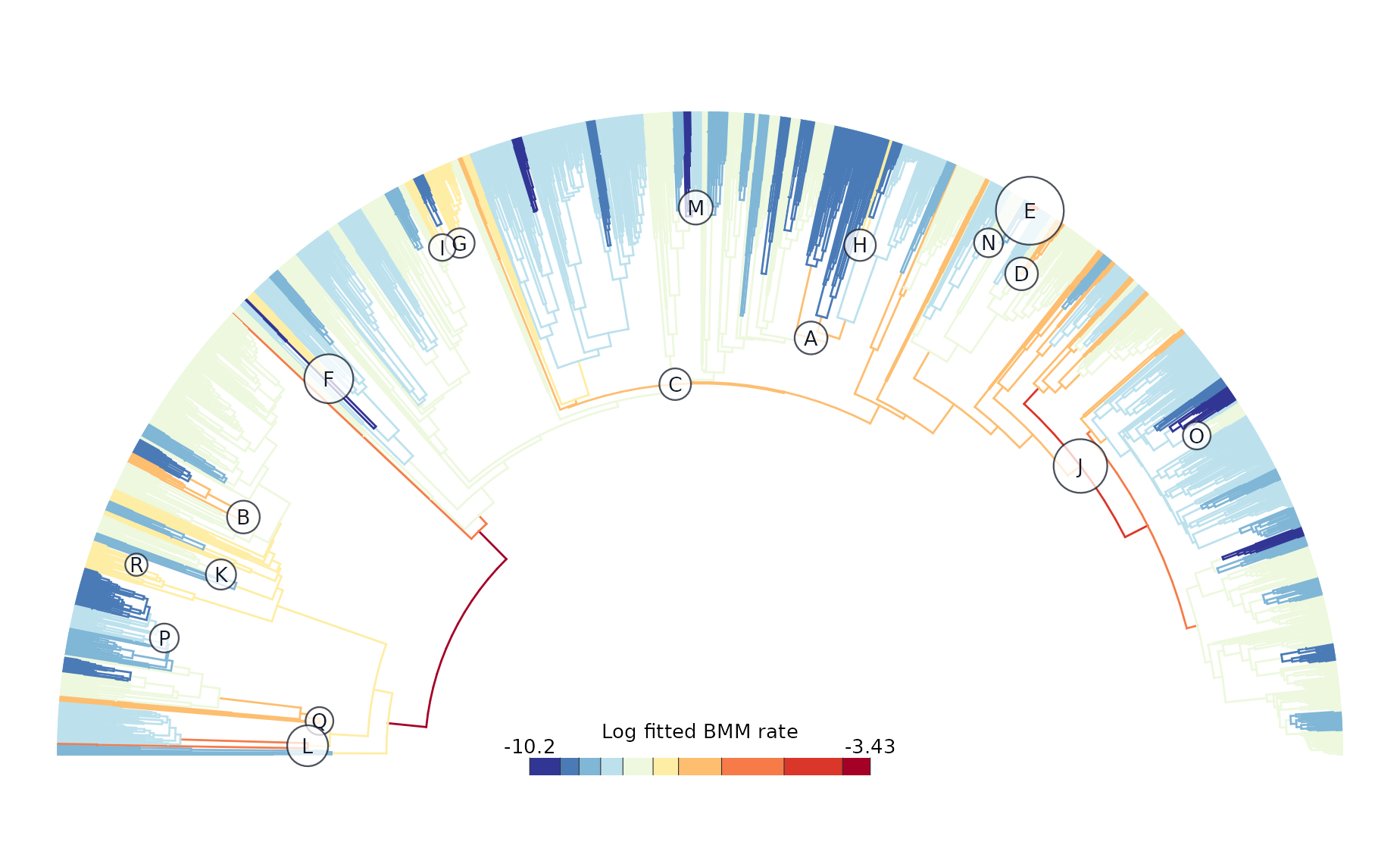
Figure 1. Focal rate-increase nodes overlaid on the Berv et al. branch-rate tree. Branch colors use the same Fisher-binned reversed RdYlBu log-rate palette as Berv et al. (2026). White lettered circles mark inferred shifts to faster fitted BMM regimes, with marker size following the square-root scaling of percent rate change used in that figure.
Fitting rate distributions
fit_rate_distribution() compares the fitted BMM regime
rates across candidate continuous models. It accepts the
bifrost_search object directly, log-transforms the positive
regime rates by default, and ranks a broad default set of
univariateML candidates.
# Fit candidate distributions to log fitted BMM regime rates.
bodyplan_rate_fit <- fit_rate_distribution(bodyplan_search)

# Precompute Gumbel bootstrap draws once; this also stores the D_KL summary.
bodyplan_rate_fit <- bootstrap_rate_distribution(
  bodyplan_rate_fit,
  model = "gumbel",
  reps = 1000,
  seed = 2026
)

# Pull out rankings, selected parameters, and the Gumbel goodness-of-fit summary.
rate_rankings <- as.data.frame(bodyplan_rate_fit, component = "rankings")
rate_parameters <- as.data.frame(
  bodyplan_rate_fit,
  component = "parameters",
  models = bodyplan_rate_fit$rankings$ml[seq_len(min(3, nrow(bodyplan_rate_fit$rankings)))]
)
rate_goodness <- as.data.frame(bodyplan_rate_fit, component = "goodness")

# Print compact previews; full tables remain in the objects above.
rate_rankings_preview <- rate_rankings[seq_len(min(5, nrow(rate_rankings))), ]
rate_parameters_preview <- rate_parameters[
  rate_parameters$selected,
  !names(rate_parameters) %in% c("selected_AIC", "selected_BIC"),
  drop = FALSE
]

print(rate_rankings_preview)
#>                    model     ml   AIC   BIC   d_AIC  d_BIC
#> 1                 Gumbel gumbel 240.7 245.6  0.0000  0.000
#> 2 Skew Generalized Error   sged 240.9 250.6  0.1814  5.019
#> 3         Skew Student-t   sstd 241.5 251.2  0.7679  5.606
#> 4            Skew Normal  snorm 244.7 251.9  3.9560  6.375
#> 5              Student-t    std 259.1 266.3 18.3200 20.740
cat("\n\n")
print(rate_parameters_preview)
#>    model distribution parameter estimate selected
#> 1 gumbel       Gumbel        mu  -8.8380     TRUE
#> 2 gumbel       Gumbel     sigma   0.8301     TRUE
cat("\n\n")
print(rate_goodness)
#>    model statistic estimate conf_low conf_high conf_level bootstrap_reps
#> 1 gumbel       DKL  0.03106  0.01314    0.1422       0.95           1000
The preview keeps the top candidate distributions, parameter
estimates for the selected Gumbel fit, and the bootstrapped
Kullback-Leibler divergence (D_KL) for the Gumbel overlay.
Use
as.data.frame(bodyplan_rate_fit, component = "rankings") or
component = "parameters" to inspect the complete
model-selection tables.
The histogram below reuses the Fisher breaks and branch-rate palette
from Figure 1. fit_rate_distribution() stores the fitted
candidates and rankings; bootstrap_rate_distribution() adds
the reproducible Gumbel bootstrap draws that plot()
displays.
# Plot the fitted Gumbel density with its stored bootstrap uncertainty.
plot(
  bodyplan_rate_fit,
  model = "gumbel",
  bootstrap = TRUE,
  bootstrap_curves = 120,
  breaks = bodyplan_rate_breaks,
  hist_col = bodyplan_rate_palette
)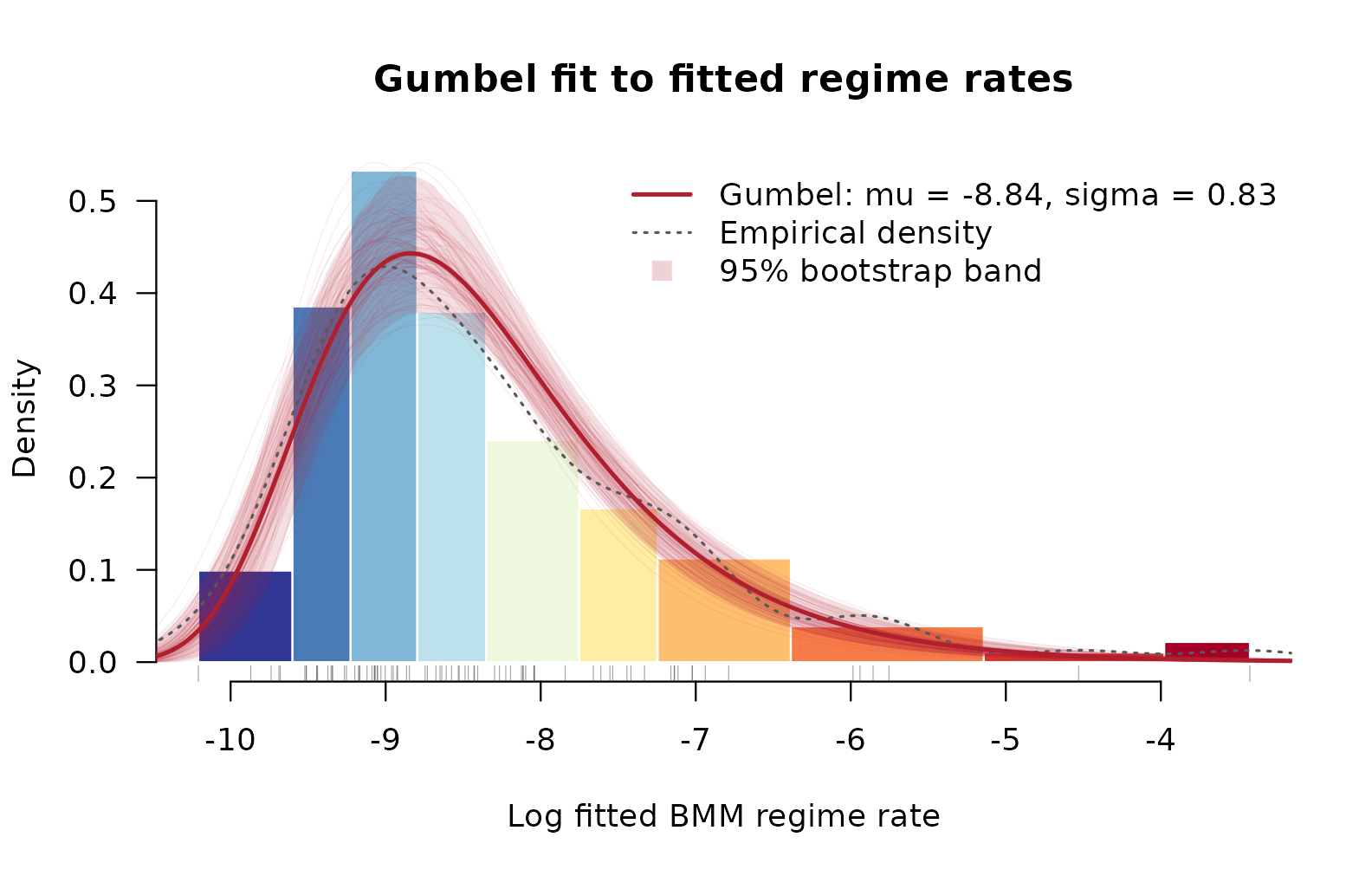
Figure 2. Fitted Gumbel distribution for the focal BMM regime rates. Histogram bars use Fisher breaks and the reversed RdYlBu palette used for branch-rate bins in Berv et al. (2026). The red line is the maximum-likelihood Gumbel density, the gray dashed curve is the empirical density, tick marks show fitted regime rates, the pale band is the pointwise 95% bootstrap interval, and thin red curves show bootstrap density draws.
Waiting times between shifts
shift_waiting_times() computes the waiting-time views
used to separate tree-wide burstiness from lineage-level shift
histories. Berv et al. (2026) report two distributional summaries:
whole-tree chronological waiting times between successive shifts, and
root-to-tip lineage waiting times used for per-lineage candidate fits.
The acceleration summary isolates increase-to-increase gaps; we print it
as context, not as the primary reported waiting-time distribution.
# Compute global, lineage-level, and acceleration waiting-time summaries.
bodyplan_waiting_times <- shift_waiting_times(bodyplan_search)

# Print the compact summaries rather than the full lineage table.
bodyplan_waiting_times$summaries$global
#>               Category      Mean   Median  Variance Count
#> 1                other 4.7537640 4.753764        NA     1
#> 2 decrease_to_decrease 0.4072759 0.242733 0.5831287    48
#> 3 decrease_to_increase 0.4507928 0.265952 0.3542168    16
#> 4 increase_to_decrease 0.4403122 0.268102 0.3722976    15
#> 5 increase_to_increase 3.1860865 3.186087 7.2261611     2
bodyplan_waiting_times$summaries$lineage
#>               Category      Mean    Median Variance Count
#> 1 decrease_to_decrease  4.878764  1.385098 44.24708  3422
#> 2 decrease_to_increase  6.824821  5.615454 23.34086  1843
#> 3 increase_to_increase 13.117374 13.117374  0.00000   550
#> 4 increase_to_decrease  4.958275  3.136740 28.88695  1642
bodyplan_waiting_times$acceleration$summary
#>            summary   n     mean   median       sd
#> 1 lineage_weighted 808 13.61213 13.11737 4.461476
#> 2        collapsed   9 19.34903 20.49203 8.152022
In Berv et al. (2026), the whole-tree chronological waits support the Weibull result for shift timing across the phylogeny, while the lineage waits support the per-lineage Exponential result for tip-to-root paths.
Fitting waiting-time distributions
The first fit below repeats the whole-phylogeny comparison from Berv et al. (2026): chronological waiting times between successive shifts are compared across the same positive-support candidate models.
# Fit positive-support candidates to whole-tree chronological waiting times.
# The default includes the initial root-to-first-shift interval.
bodyplan_waiting_fit <- fit_waiting_time_distribution(
  bodyplan_waiting_times,
  global_include_root_wait = TRUE
)

# Extract rankings plus parameters for the top-supported candidates.
waiting_rankings <- as.data.frame(bodyplan_waiting_fit, component = "rankings")
waiting_parameters <- as.data.frame(
  bodyplan_waiting_fit,
  component = "parameters",
  models = bodyplan_waiting_fit$rankings$ml[seq_len(min(3, nrow(bodyplan_waiting_fit$rankings)))]
)

# Print compact previews; full tables remain in the fitted object.
waiting_rankings_preview <- waiting_rankings[
  seq_len(min(5, nrow(waiting_rankings))),
  ,
  drop = FALSE
]
waiting_parameters_preview <- waiting_parameters[
  waiting_parameters$selected,
  !names(waiting_parameters) %in% c("selected_AIC", "selected_BIC"),
  drop = FALSE
]

print(waiting_rankings_preview)
#>              model       ml    AIC    BIC   d_AIC   d_BIC
#> 1          Weibull  weibull  54.45  59.27   0.000   0.000
#> 2            Gamma    gamma  60.04  64.85   5.583   5.583
#> 3        Lognormal    lnorm  63.71  68.52   9.256   9.256
#> 4      Exponential      exp  65.73  68.14  11.280   8.869
#> 5 Inverse Gaussian invgauss 287.80 292.60 233.300 233.300
cat("\n\n")
print(waiting_parameters_preview)
#>     model distribution parameter estimate selected
#> 1 weibull      Weibull     shape   0.7701     TRUE
#> 2 weibull      Weibull     scale   0.4495     TRUE
Set global_include_root_wait = FALSE when you need to
mirror the archived TimeToNext[-1] check rather than the
reported whole-tree Weibull summary.
Setting by_lineage = TRUE repeats the candidate-model
comparison for each lineage with enough waiting-time observations. These
fits provide the compact-data check for the Berv et al. (2026) statement
that most tip-to-root paths favor a constant-rate Exponential
waiting-time model.
# Repeat the waiting-time fits independently for each lineage.
bodyplan_lineage_waiting_fit <- fit_waiting_time_distribution(
  bodyplan_waiting_times,
  by_lineage = TRUE
)

# Summarize how many lineages had enough waiting times to fit.
lineage_summary <- as.data.frame(bodyplan_lineage_waiting_fit, component = "lineage")

lineage_fit_counts <- data.frame(
  lineages_with_waits = nrow(lineage_summary),
  fitted_lineages = sum(lineage_summary$fit_success),
  skipped_lineages = sum(!lineage_summary$fit_success)
)

fitted_lineage_summary <- lineage_summary[lineage_summary$fit_success, ]

lineage_exponential_check <- data.frame(
  criterion = c("BIC", "AIC"),
  best_model = "exp",
  exponential_lineages = c(
    sum(fitted_lineage_summary$best_BIC == "exp"),
    sum(fitted_lineage_summary$best_AIC == "exp")
  ),
  fitted_lineages = nrow(fitted_lineage_summary),
  percent_fitted = c(
    round(
      100 * sum(fitted_lineage_summary$best_BIC == "exp") /
        nrow(fitted_lineage_summary),
      1
    ),
    round(
      100 * sum(fitted_lineage_summary$best_AIC == "exp") /
        nrow(fitted_lineage_summary),
      1
    )
  ),
  reported_percent = c("86%", NA)
)

# Print the compact summaries needed for the manuscript check.
print(lineage_fit_counts)
#>   lineages_with_waits fitted_lineages skipped_lineages
#> 1                2021            1708              313
cat("\n\n")
print(lineage_exponential_check)
#>   criterion best_model exponential_lineages fitted_lineages percent_fitted
#> 1       BIC        exp                 1482            1708           86.8
#> 2       AIC        exp                 1603            1708           93.9
#>   reported_percent
#> 1              86%
#> 2             <NA>
cat("\n\n")
print(bodyplan_lineage_waiting_fit$lambda_summary)
#>      n      mean    median         sd hdi_95_low hdi_95_high
#> 1 1708 0.2008326 0.1961029 0.08901564 0.07866725   0.4027226
The reported statement that 86% of tip-to-root paths favor a constant-rate Exponential model comes from the BIC-supported per-lineage model summary in the archived workflow. The compact object gives 1,482 BIC Exponential winners among 1,708 fitted lineage paths, or 86.8%, while AIC gives a higher count of 1,603 Exponential winners, or 93.9%. We print both criteria to make that distinction explicit; the small difference between the compact BIC percentage and the published 86% reflects reported-value rounding/truncation or full-archive run details.
The full per-lineage model-count and parameter tables remain
available with
as.data.frame(bodyplan_lineage_waiting_fit, component = "lineage")
and component = "lineage_parameters"; here we print only
the compact summaries needed to check the reported 86% statement. The
lambda_summary table includes the mean, median, standard
deviation, and a 95% shortest-interval summary for the lineage-level
Exponential rate parameter.
Practical Takeaways
-
shift_transitions()extracts fitted parent-child regime changes from the focal BMM map and records timing, direction, and signed rate differences. -
rateMap()provides the Berv et al. (2026) branch-rate tree;shift_node_marks()can optionally use drop-oneic_weightsto flag low-support shifts. -
shift_node_marks()prepares rate-increase annotations, andplot()overlays them on an existing tree plot without rebuilding the branch-rate layer. -
fit_rate_distribution()wrapsunivariateML::model_select()for fitted BMM regime rates andplot(rate_fit, model = "gumbel")draws the Berv et al. (2026)-style Gumbel overlay. -
shift_waiting_times()computes global, lineage-level, and acceleration-focused waiting-time summaries from the compact focal object. -
fit_waiting_time_distribution()supports both whole-tree chronological waits and per-lineage waiting-time fits used to check the Berv et al. (2026) Weibull and Exponential summaries. - Part 4 uses
compare_shift_magnitudes()and the compact sensitivity bundle to compare log absolute rate-change magnitudes for increases and decreases. - Part 5 reuses the temporal regime framework for post-hoc integration summaries, not for spatial/local assemblage covariance.
- Use the complete Berv et al. (2026) archive for proposal-level history, candidate model fits, and external ecological metadata; use the compact focal object for these timing and distribution summaries.
References
If you use these data or reproduce this workflow, the most relevant citations are:
- Berv, Jacob S., Charlotte M. Probst, Santiago Claramunt, J. Ryan Shipley, Matt Friedman, Stephen A. Smith, David F. Fouhey, and Brian C. Weeks. 2026. “Rates of passerine body plan evolution in time and space.” Nature Ecology & Evolution. https://doi.org/10.1038/s41559-026-03110-5
- Berv, Jacob S., Charlotte M. Probst, Santiago Claramunt, J. Ryan Shipley, Matt Friedman, Stephen A. Smith, David F. Fouhey, and Brian C. Weeks. 2026. “Supplementary data archive for Rates of passerine body plan evolution in time and space” (v1.0.0) [Data set]. Zenodo. https://doi.org/10.5281/zenodo.19198393
- Claramunt, Santiago, Christopher Sheard, Joseph W. Brown, Guillermo Cortes-Ramirez, Joel Cracraft, Mason M. Su, Brian C. Weeks, and Joseph A. Tobias. 2025. “A new time tree of birds reveals the interplay between dispersal, geographic range size, and diversification.” Current Biology. Advance online publication. https://doi.org/10.1016/j.cub.2025.07.004
Software Used in This Vignette
-
bifrostfor transition extraction, shift waiting times, rate-map helpers, and distribution-fitting wrappers. -
apeandphytoolsunderlie the mapped-tree calculations in these summaries. -
classIntcomputes the Fisher breaks for the rate-distribution histogram. -
RColorBrewersupplies the Berv et al. (2026) branch-rate palette. -
univariateMLfits candidate distributions when these examples run. -
evdevaluates the fitted Gumbel density for the rate-distribution overlay.