Whole-Tree Models, PCA, and bifrost

Introduction

This vignette builds on the Brownian-motion and covariance background developed in Brownian Motion and Multivariate Shifts. It considers how BM, OU, and EB behave as whole-tree models, what happens when empirical datasets are more heterogeneous than those single-process descriptions allow, and where bifrost sits within that broader landscape.

Whole-tree models are useful because they provide simple ways to describe how variation accumulates across a phylogeny. But that simplicity can also become a limitation when different parts of the tree follow different local regimes, since a single fit may average over structure that is biologically important. PCA often enters this discussion as an appealing way to simplify multivariate data, yet its leading axes are chosen to maximize sample variance rather than preserve the evolutionary structure we necessarily care about. The goal here is to clarify what whole-tree models capture, what they can obscure, and why PCA is not a neutral substitute for modeling heterogeneity directly.

1. BM, OU, EB, and the limits of whole-tree models

Model	Core idea	Main parameters	Typical biological reading
BM	Diffusion with no preferred direction and constant rate through time	$\sigma^2$	Trait variance accumulates steadily as lineages diverge
OU	Diffusion plus pull toward an optimum	$\alpha$ , $\theta$ , $\sigma^2$	Traits wander, but are restrained around an adaptive peak
EB	Diffusion with a systematic tempo change through time	$\sigma_0^2$ , $r$	Evolution is fastest early and then slows, or more generally speeds up or slows down through time

Under BM, variance accumulates linearly with time and no optimum is preferred. That makes BM a useful baseline for asking whether a multivariate rate structure is constant across a tree. When bifrost searches for branch-specific shifts under BM/BMM, it is still working inside that diffusion-based family.

OU changes the story by adding deterministic pull toward an optimum. The parameter $\alpha$ controls how strongly lineages are drawn back toward $\theta$ , so OU is often read as a simple model of adaptive constraint or stabilization (Hansen 1997; Butler and King 2004). EB is different again: it is not about attraction to an optimum, but about a directional change in tempo through time, often written as a rate like $\sigma^2(t) = \sigma_0^2 e^{rt}$ , with classic early-burst behavior corresponding to $r < 0$ (Harmon et al. 2010).

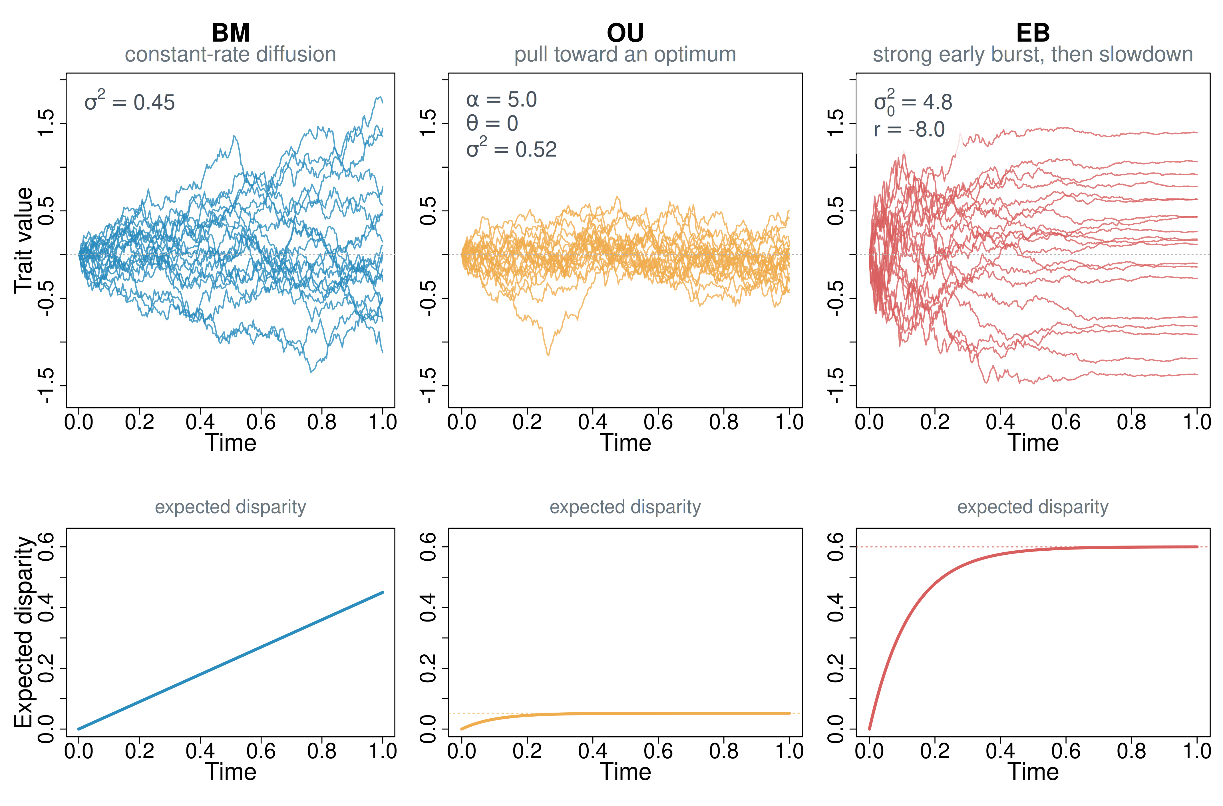
Six panels arranged in two rows and three columns. Top row shows BM, OU, and EB simulated trajectories through time. Bottom row shows the corresponding theoretical expected disparity curves: BM rises linearly, OU rises then plateaus, and EB rises quickly early and then flattens.

Figure 1. Three simple continuous-trait models contrasted with simulations and their theoretical disparity implications. Top row: simulated trajectories under BM, OU, and EB. BM diffuses at a constant rate, so trajectories spread steadily through time. OU adds deterministic pull toward an optimum, which keeps trajectories more tightly bounded around the center. EB begins with a stronger early burst and then slows sharply, so most divergence is front-loaded. Bottom row: the corresponding theoretical expected disparity-through-time curves under the same parameter values. BM increases linearly, OU rises and saturates, and EB accumulates disparity early before flattening.

Figure 1 also clarifies the scope of these models. BM, OU, and EB each provide a coarse whole-tree summary of how variation accumulates: BM assumes one diffusion process across the tree, OU adds one global pull structure, and EB allows one simple tree-wide trend in tempo. If a dataset instead contains patchy clade-specific shifts, mixtures of slower and faster regimes, or several distinct episodes of change, then even these more flexible whole-tree descriptions can miss the signal. EB is the clearest example: it allows non-uniformity, but only as one smooth tree-wide tempo trend rather than as localized shifts.

2. When the process is heterogeneous across the tree

That kind of mismatch is where bifrost becomes useful. The package does not replace BM with a different global family. Instead, it keeps the local process Brownian and allows different parts of the tree to occupy different multivariate BM/BMM regimes. In that sense, variation across an empirical tree can be approximated as a multi-regime Gaussian/Brownian process on a painted phylogeny: within each regime, traits still evolve as multivariate Gaussian diffusion, but across the tree the observed pattern can reflect several branch- or clade-specific regimes rather than one uniform model for the entire dataset.

This matters because heterogeneity is not only a problem for whole-tree fits. If the underlying process is patchy, nested, or recurrent across the phylogeny, then even models assigned to large clades can still average over mixed local regimes and provide a poor description of the data. Figure 2 extends the simpler descendant-clade shift logic introduced in Brownian Motion and Multivariate Shifts to that more heterogeneous setting.

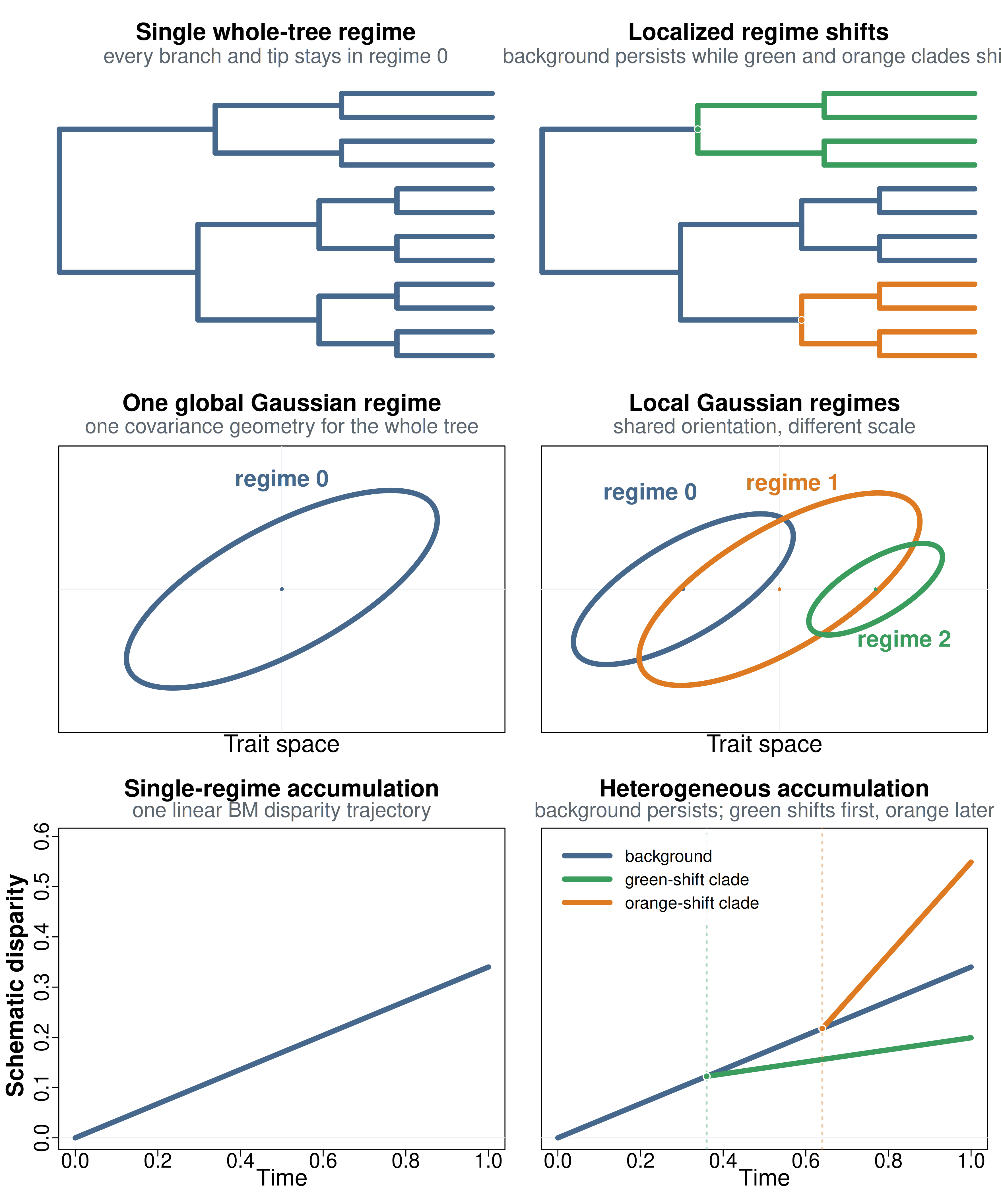
Six-panel schematic figure in three rows and two columns. Left column shows a single-regime phylogeny, one global Gaussian ellipse in trait space, and one linear disparity-accumulation curve. Right column shows a phylogeny with two localized shift clades, three Gaussian covariance ellipses with shared orientation but different size, and several clade-specific piecewise disparity curves.

Figure 2. Whole-tree summaries versus heterogeneous regime mixtures. Left column: one global BM/BMM regime applies everywhere, yielding one tree-wide Gaussian trait-space geometry and one linear disparity-accumulation pattern. Right column: localized clade-specific shifts create multiple regimes across the tree; under bifrost’s current assumptions those local regimes remain multivariate Gaussian with shared covariance geometry but different scale, and their disparity accumulation patterns can diverge after shifts. Horizontal offsets in the trait-space panel are only for visual separation, not different regime means. Those local trajectories need not be well summarized by any single whole-tree fit.

This perspective is close in spirit to mixed Gaussian phylogenetic model frameworks such as PCMFit, which also allow different Gaussian evolutionary descriptions to be assigned to different parts of a tree and search among alternative shift configurations (Mitov, Bartoszek, and Stadler 2019; Mitov et al. 2020). The main distinction is that bifrost is currently narrower and more directly oriented toward high-dimensional original trait data. It keeps the local process within the multivariate BM/BMM family, fits regime structure directly in trait space through penalized multivariate GLS, and assumes proportional regime scaling rather than the broader class of Gaussian shift models considered in PCMFit. Because bifrost fits heterogeneous regime structure directly, it can capture much more complex rate-shift patterns than a single whole-tree BM, OU, or EB fit while still remaining inside a Brownian, covariance-based framework.

bayou is another nearby comparison (Uyeda and Harmon 2014), but it addresses a different kind of heterogeneity: OU adaptive-regime shifts rather than the multivariate BM/BMM rate shifts targeted by bifrost. Multivariate OU models remain an important area of method development (Mariadassou, Lambert, and Morlon 2018), whereas bifrost’s current niche is heterogeneous multivariate BM/BMM with branch-level rate shifts under proportional regime scaling.

3. PCA Is Not a Neutral Fix

When multivariate data are high-dimensional and difficult to summarize directly, one common response is to simplify them first, usually with PCA, rather than model the heterogeneity itself. That can be useful for visualization and exploratory summaries, but it is not a neutral preprocessing step for comparative inference (Revell 2009; Uyeda, Caetano, and Pennell 2015). PCA can hide the axes carrying the biologically relevant difference, and it can also reorder axes in ways that change which global model looks best supported (Uyeda, Caetano, and Pennell 2015).

Why PCA Truncation Can Mislead

The first of those problems is geometric. PCA orders axes by realized sample variance, not by whether they contain the biologically relevant contrast. If the process of interest lies partly along a lower-variance direction, then truncating to the leading PC can discard the very signal we want to interpret, a point long recognized more generally in the PCA literature (Jolliffe 1982). This is easiest to see in a simple two-regime example where most variation lies along one axis, but the important difference lies along another.

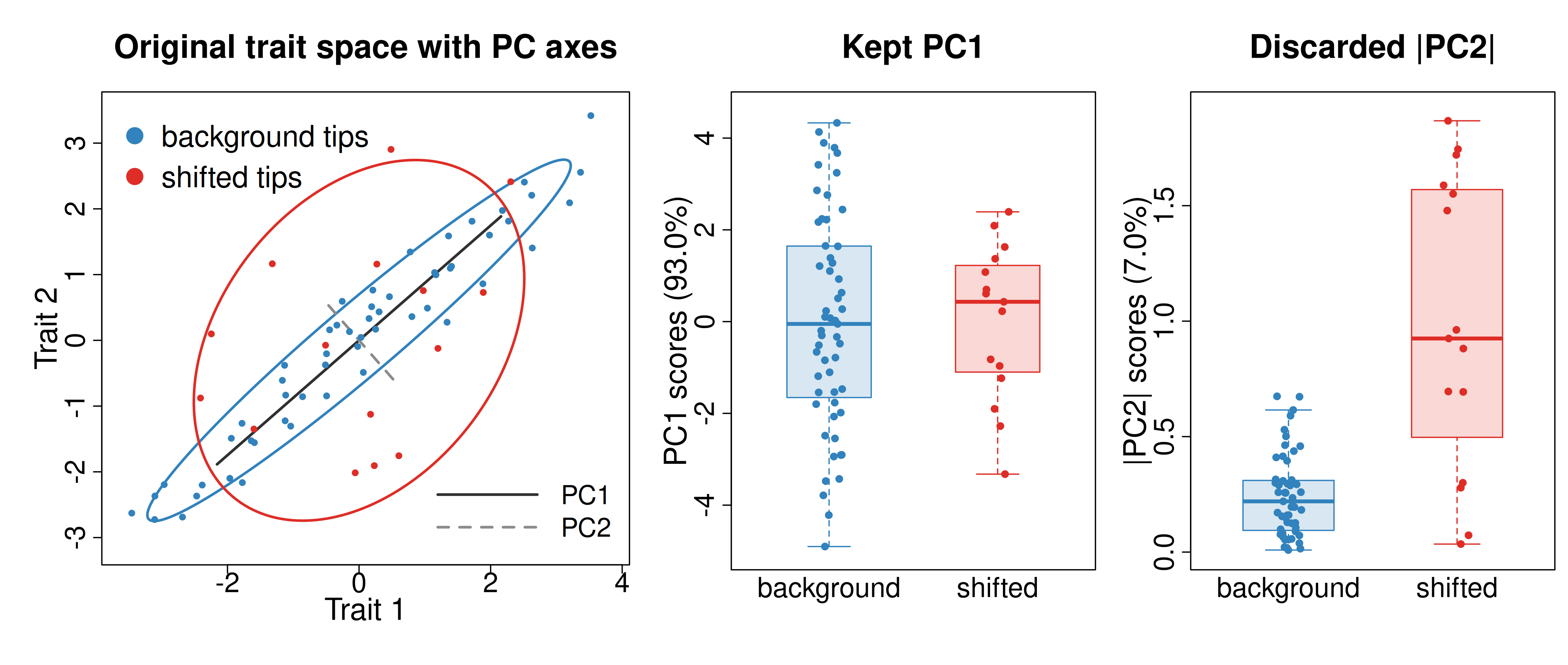
Three-panel figure arranged left to right. Left: two centered diagonal trait clouds with similar major-axis spread but different minor-axis spread, with principal-component axes overlaid. Middle: vertical boxplots and points for retained PC1 scores, showing strong overlap between regimes. Right: vertical boxplots and points for absolute PC2 scores, showing the shifted regime is much broader on the discarded axis.

Figure 3. Why truncating PCA can mislead. Left: both regimes share the same broad diagonal axis of variation, but the shifted regime has much greater spread perpendicular to that axis; the overlaid lines show PC1 and PC2. Middle: scores on retained PC1 overlap strongly even though PC1 captures most total variance. Right: the regime difference is clear on the discarded low-variance axis, shown here as absolute distance on PC2 because the difference is in spread rather than mean.

Here both regimes share the same broad major axis, but the shifted regime has much greater variance along the lower-variance axis perpendicular to it. PCA still assigns 93.0% of the total sample spread to PC1 because that long diagonal axis dominates the variance budget. Yet the retained PC1 scores overlap strongly, while the discarded |PC2| scores are exactly where the regime difference becomes clear. Because the shift is in spread rather than mean, the contrast appears in |PC2| rather than in signed PC2 scores.

Phylogenetic PCA can be more coherent than ordinary PCA under a Brownian-motion null, but it is still a model-based rotation rather than a neutral preprocessing step (Revell 2009; Uyeda, Caetano, and Pennell 2015).

PCA Can Distort Model Selection

The truncation problem above is only one PCA caution. A second issue is more inferential: PCA can change which comparative model appears best supported. In the simulations of Uyeda, Caetano, and Pennell (2015), even when all traits truly evolved under constant-rate multivariate BM, the first few standard PC axes often looked as though they were better fit by an early-burst model. The point is not that PCA invents an early burst out of thin air; it is that ranking axes by realized sample variance across the whole tree can privilege combinations of traits with unusually large deep divergences.

We show a compact illustration of this result using a reduced version of the equal-rate BM setup discussed in Uyeda, Caetano, and Pennell (2015): 20 replicate pure-birth trees with 50 tips, 20 independent BM traits, and BM, OU, and EB model fits to both the original traits and the first six standard PC scores.

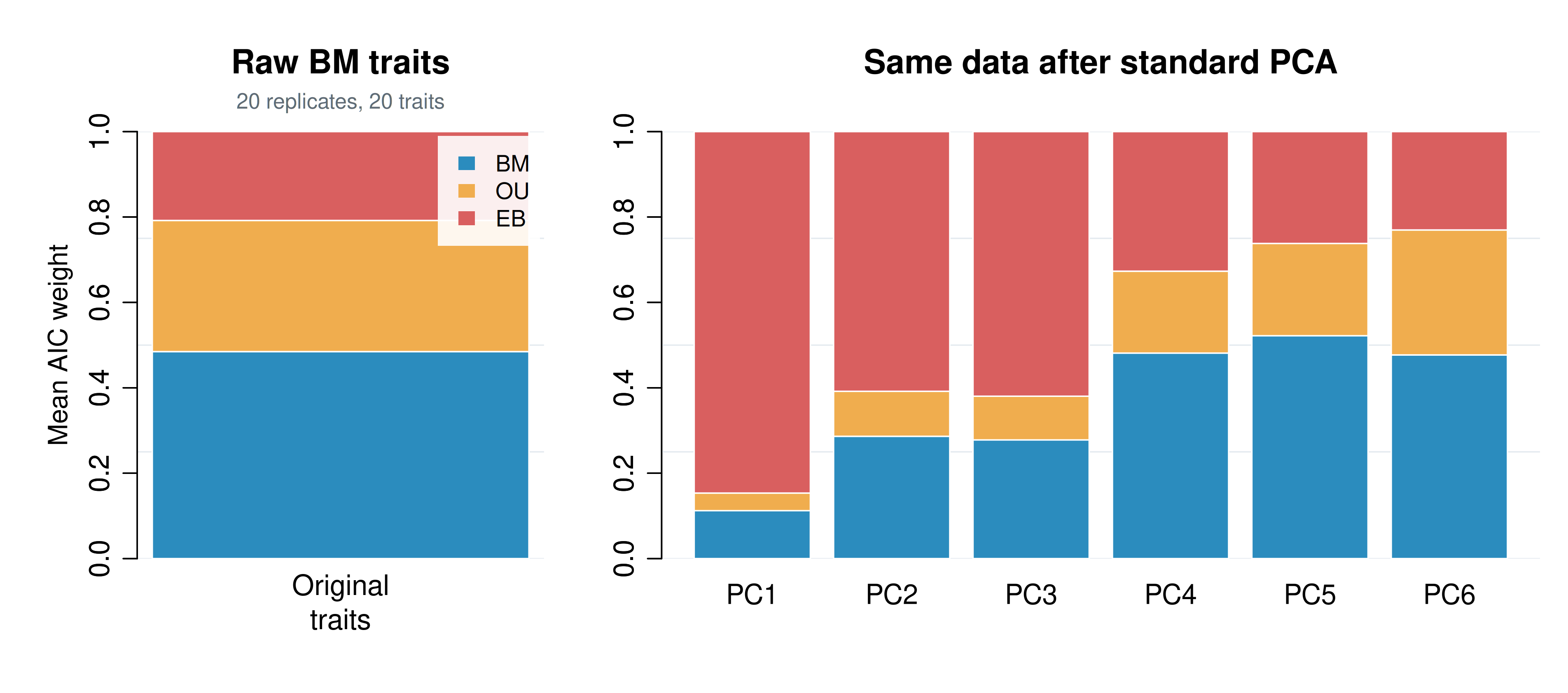
Two-panel figure. Left: one stacked bar for original traits with the largest segment labeled BM and smaller OU and EB segments. Right: six stacked bars labeled PC1 through PC6, with large EB segments on the earliest bars and more BM support on later bars.

Figure 4. A compact illustration of the standard-PCA artifact emphasized by Uyeda, Caetano, and Pennell (2015). Left: averaged across the original traits, BM has the highest support. Right: after standard PCA, support is pulled toward EB on the earliest axes even though the generating process was BM throughout.

The PCA issue here is different from the truncation problem above. The signal is not being hidden on a low-variance axis. Instead, standard PCA changes which univariate combinations get placed first. Averaged across the original BM traits, BM remains the best-supported model, although its mean AIC weight does not approach 1 because OU and EB collapse onto BM when their extra parameter is unnecessary; under this three-model comparison, the BM ceiling is only about 0.58, as Uyeda et al. discuss. After standard PCA, the leading axes are no longer a neutral sample from the multivariate process: they are the axes most likely to make a constant-rate BM data set look EB-like.

PCA can be useful descriptively, but once the transformed axes are treated as the units of model comparison, the ranking itself can change which macroevolutionary explanations look plausible. PCA is a variance-maximizing dimension reduction, not a model of tree-structured heterogeneity. It therefore does not rescue a heterogeneous dataset from the limitations of a single whole-tree fit; it can add another layer of distortion on top of that original mismatch. That is why bifrost fits models in the original trait space and treats PCA as optional description rather than as primary preprocessing for inference.

4. Mapping Theory to the `bifrost` API

With that in mind, the main package interface becomes easier to read. bifrost is most useful when a single whole-tree summary is too crude, but a Brownian, covariance-based description is still a reasonable local approximation within regimes. Relative to broader mixed-Gaussian frameworks such as PCMFit, it trades model generality for tractability in high-dimensional original trait space.

bifrost handles high-dimensional trait data through penalized-likelihood multivariate GLS fits implemented in mvMORPH::mvgls (Clavel, Aristide, and Morlon 2019). In ordinary multivariate GLS, covariance estimation becomes unstable or singular when the number of traits is large relative to the number of species. Penalization regularizes those covariance estimates, which makes it possible to work directly in the original trait space rather than collapsing the data to a few PCs first. In bifrost, that high-dimensional machinery is combined with proportional regime scaling, which further keeps the BM/BMM search tractable.

Theoretical idea	`bifrost` component	Interpretation
Single-regime baseline process	`baseline_tree`, `formula`, `baseline_ic`	One multivariate BM model shared across the tree
Candidate evolutionary shift	internal nodes passing `min_descendant_tips`	A descendant clade is allowed to have a different regime
Model comparison	`IC`, `shift_acceptance_threshold`, `optimal_ic`	Controls how much better a more complex model must fit
Regime-specific rate structure	`VCVs`	Estimated regime-specific variance-covariance matrices, interpreted in the current model through proportional scaling across regimes
Support for accepted shifts	`ic_weights`	Drop-one support values for shifts in the final model
Search dynamics	`model_fit_history`	Sequence of accepted and rejected candidates

library(bifrost)

fit <- searchOptimalConfiguration(
  baseline_tree              = tree,
  trait_data                 = trait_data,
  formula                    = "trait_data ~ 1",
  min_descendant_tips        = 10,
  num_cores                  = 4,
  shift_acceptance_threshold = 20,
  uncertaintyweights_par     = TRUE,
  IC                         = "GIC",
  method                     = "H&L",
  error                      = TRUE,
  plot                       = FALSE
)

fit$shift_nodes_no_uncertainty
fit$VCVs
fit$ic_weights

For intercept-only morphometric datasets, formula = "trait_data ~ 1" corresponds to the multivariate BM/BMM case discussed in Part 1, Brownian Motion and Multivariate Shifts. At present, that means BM/BMM fits with proportional regime scaling rather than arbitrary covariance reorientation across clades. For multivariate pGLS-style analyses with predictors, the same logic applies except that the covariance model now describes residual structure after accounting for the predictors.

Practical Takeaways

BM, OU, and EB are useful whole-tree summaries, but they can fit heterogeneous datasets poorly when local regimes are nested, patchy, or clade-specific.
bifrost addresses that problem by fitting heterogeneous multivariate BM/BMM regimes directly in the original trait space, using penalized multivariate GLS to remain tractable for high-dimensional data.
PCA is useful descriptively, but its axes maximize sample variance rather than preserve the evolutionary structure we necessarily care about.
PCA can mislead inference in more than one way: truncation can discard biologically relevant low-variance structure, and axis ranking can make different comparative models look spuriously attractive.
bifrost therefore treats PCA as optional description rather than required preprocessing, and its current niche is multivariate BM/BMM shift detection under proportional regime scaling.

Next Steps

If you want to connect this back to the broader theoretical setup or a worked analysis:

Part 1, Brownian Motion and Multivariate Shifts, lays out the BM and covariance ideas assumed here;
the jaw-shape vignette shows a full morphometric workflow on a real dataset.

References

Butler, M. A., and King, A. A. (2004). Phylogenetic Comparative Analysis: A Modeling Approach for Adaptive Evolution. https://doi.org/10.1086/426002
Clavel, J., Aristide, L., and Morlon, H. (2019). A Penalized Likelihood Framework for High-Dimensional Phylogenetic Comparative Methods and an Application to New-World Monkeys Brain Evolution. https://doi.org/10.1093/sysbio/syy045
Hansen, T. F. (1997). Stabilizing Selection and the Comparative Analysis of Adaptation. https://doi.org/10.1111/j.1558-5646.1997.tb01457.x
Harmon, L. J., Losos, J. B., Davies, T. J., Gillespie, R. G., Gittleman, J. L., Jennings, W. B., Kozak, K. H., McPeek, M. A., Moreno-Roark, F., Near, T. J., Purvis, A., Ricklefs, R. E., Schluter, D., Schulte II, J. A., Seehausen, O., Sidlauskas, B. L., Torres-Carvajal, O., Weir, J. T., and Mooers, A. O. (2010). Early Bursts of Body Size and Shape Evolution Are Rare in Comparative Data. https://doi.org/10.1111/j.1558-5646.2010.01025.x
Jolliffe, I. T. (1982). A Note on the Use of Principal Components in Regression. https://doi.org/10.2307/2348005
Mariadassou, M., Lambert, A., and Morlon, H. (2018). Inference of Adaptive Shifts for Multivariate Correlated Traits. https://doi.org/10.1093/sysbio/syy005
Mitov, V., Bartoszek, K., and Stadler, T. (2019). Automatic Generation of Evolutionary Hypotheses Using Mixed Gaussian Phylogenetic Models. https://doi.org/10.1073/pnas.1813823116
Mitov, V., Bartoszek, K., Asimomitis, G., and Stadler, T. (2020). Fast Likelihood Calculation for Multivariate Gaussian Phylogenetic Models with Shifts. https://doi.org/10.1016/j.tpb.2019.11.005
Revell, L. J. (2009). Size-Correction and Principal Components for Interspecific Comparative Studies. https://doi.org/10.1111/j.1558-5646.2009.00804.x
Uyeda, J. C., and Harmon, L. J. (2014). A Novel Bayesian Method for Inferring and Interpreting the Dynamics of Adaptive Landscapes from Phylogenetic Comparative Data. https://doi.org/10.1093/sysbio/syu057
Uyeda, J. C., Caetano, D. S., and Pennell, M. W. (2015). Comparative Analysis of Principal Components Can Be Misleading. https://doi.org/10.1093/sysbio/syv019

Software Used in This Vignette

Ho, L. S. T., and Ané, C. (2014). A Linear-Time Algorithm for Gaussian and Non-Gaussian Trait Evolution Models. Systematic Biology, 63(3), 397-408. [phylolm]
Clavel, J., Escarguel, G., and Merceron, G. (2015). mvMORPH: an R package for fitting multivariate evolutionary models to morphometric data. Methods in Ecology and Evolution, 6(11), 1311-1319. https://doi.org/10.1111/2041-210X.12420
Paradis, E., and Schliep, K. (2019). ape 5.0: an environment for modern phylogenetics and evolutionary analyses in R. Bioinformatics, 35, 526-528. https://doi.org/10.1093/bioinformatics/bty633
Revell, L. J. (2024). phytools 2.0: an updated R ecosystem for phylogenetic comparative methods (and other things). PeerJ, 12, e16505. https://doi.org/10.7717/peerj.16505

AI Assistance

This vignette was developed with assistance from OpenAI tools for drafting, editing, and figure refinement; all scientific content, interpretation, and final decisions were reviewed by the authors.