Brownian Motion and Multivariate Shifts

Introduction

This vignette introduces the Brownian-motion-based theory behind bifrost. The applied vignettes show full analyses on real datasets; the goal here is to develop the underlying ideas and the intuition behind them. Whole-Tree Models, PCA, and bifrost takes up the model-selection side of the story.

At a high level, bifrost rests on three ideas:

1. trait evolution is modeled as a stochastic process on a phylogeny,
2. most empirical datasets are multivariate, so covariance matters as much as rate, and
3. branch-specific shifts are interesting because they let the multivariate rate structure change across the tree.

bifrost is built around Brownian-motion-based models, so most of what follows focuses on that family. Within that family, the current search is narrower than the full conceptual space described below: it targets branch-specific proportional scaling of a shared covariance geometry.

1. Why Stochastic Models?

Comparative datasets record the outcomes of many small processes acting over long stretches of time: mutation, drift, development, integration among traits, and changing environments. We rarely observe those microscopic steps directly. Instead, we model the distribution of possible outcomes.

That is the value of a stochastic model. It does not claim that evolution is unstructured. Instead, it treats uncertainty as something that can still be described with parameters. In comparative biology, those parameters usually control:

• an ancestral state or intercept,
• the rate at which variance accumulates through time, and
• the covariance structure among traits, together with the phylogenetically induced covariance among species.

The phylogeny is what makes this a comparative model rather than a generic random process. Branch lengths encode time, and shared ancestry tells us which species should be statistically similar before we even look at the trait matrix.

2. Brownian Motion on a Phylogeny

The simplest continuous-trait model is Brownian motion (BM). In one dimension,

$$dX_t = \sigma dB_t,$$

where $B_t$ is standard Brownian motion and $\sigma^2$ is the evolutionary rate. Under BM, the expected trait value stays centered on its starting point while variance grows linearly with time:

$$\mathrm{Var}(X_t) = \sigma^2 t.$$

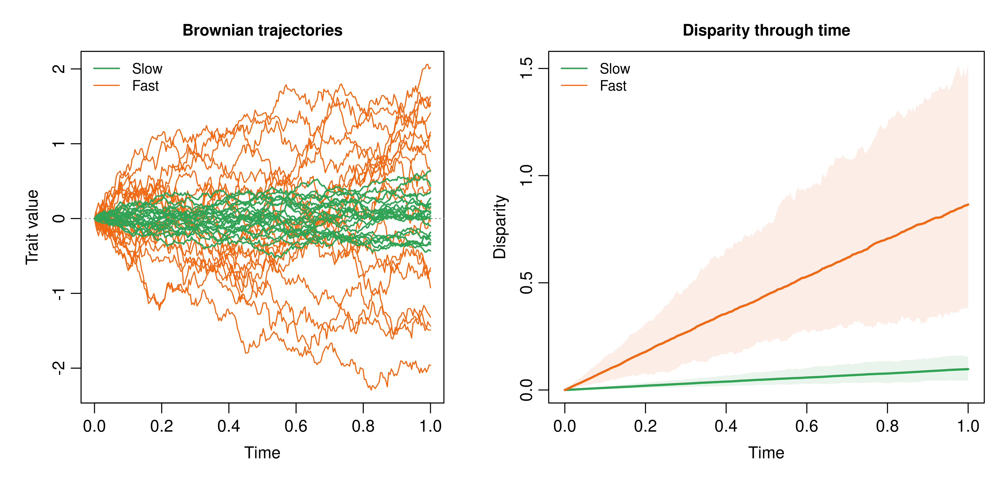
Figure 1. Brownian motion with two rates. Left: slow green trajectories $\left(\sigma^2 = 0.1\right)$ remain tightly clustered, whereas fast orange trajectories $\left(\sigma^2 = 0.9\right)$ spread more rapidly. Larger $\sigma^2$ increases diffusion, not directional tendency. Right: disparity through time. Solid colored lines show the mean sampled disparity across repeated batches of 20 trajectories, and ribbons show the central 95% range across those batches.

Interactive Brownian Rate Explorer

Adjust the two regime rates. This browser-side explorer keeps the trajectory panel lightweight while letting the disparity panel update live with the same sample size used for the displayed trajectories.

Green regimeOrange regime

Green rate 0.10

Orange rate 0.90

Trajectories

30 trajectories per regime

Disparity

70 batches; n = 30 trajectories per batch

Each slider only updates its own regime, and the disparity summary uses the same sample size as the displayed trajectory panel: 30 trajectories per regime.

On a phylogeny, BM does more than generate trait variance through time: it also implies a covariance structure among species. Following Felsenstein (1985), the covariance between species $i$ and $j$ is proportional to the amount of history they share from the root to their most recent common ancestor:

$$\mathrm{Cov}(X_i, X_j) = \sigma^2 T_{ij}.$$

That is the statistical reason close relatives tend to resemble each other under BM.

Figure 2. Phylogenetic covariance is shared history made explicit. Left: a small ultrametric tree. Right: the corresponding shared-history matrix from ape::vcv.phylo(), plotted so each heatmap row aligns vertically with the corresponding tree tip.

The shared-history matrix for this toy tree is:

round(shared_history, 2)
#>     A   B   C   D   E
#> A 2.1 1.3 0.7 0.0 0.0
#> B 1.3 2.1 0.7 0.0 0.0
#> C 0.7 0.7 2.1 0.0 0.0
#> D 0.0 0.0 0.0 2.1 1.5
#> E 0.0 0.0 0.0 1.5 2.1

BM is often described as a neutral or drift-like baseline, but that should be treated as intuition rather than a literal equivalence. A BM fit does not prove that selection was absent. It means the data are consistent with stochastic diffusion whose covariance is fully structured by the phylogeny.

3. From One Trait to Many

Most morphological and ecological datasets are not truly univariate. Landmarks, skeletal dimensions, climatic niches, and life-history syndromes all involve traits that can change together.

The natural multivariate extension of BM starts with trait-level covariance in $\mathbf{\Sigma}$, then leads to proportional rate shifts, higher-dimensional eigenvalue structure, and finally the full phylogenetic covariance $\mathbf{C} \otimes \mathbf{\Sigma}$.

At the simplest level, that extension replaces a single rate parameter with a variance-covariance matrix:

$$\mathbf{\Sigma} = \begin{bmatrix} \sigma^2_1 & \sigma_{12} & \cdots \\ \sigma_{21} & \sigma^2_2 & \cdots \\ \vdots & \vdots & \ddots \end{bmatrix}.$$

The diagonal entries are trait-specific rates, and the off-diagonal entries are evolutionary covariances. In other words, the diagonal tells us how quickly each trait changes, while the off-diagonal tells us whether traits tend to change together.

Covariance geometry

One useful way to compare two matrices is by their eigenstructure. In the Flury hierarchy, the strongest similarity is equality; a weaker but still structured relationship is proportionality, where one matrix is just a scalar multiple of another; another is the common principal components (CPC) case, where matrices share their major axes but not necessarily the same eigenvalues; and a stronger difference changes both eigenvectors and eigenvalues (Phillips and Arnold 1999). As a rough visual guide, ellipse orientation reflects correlation structure, whereas ellipse size reflects overall rate (Stepanova et al. 2025).

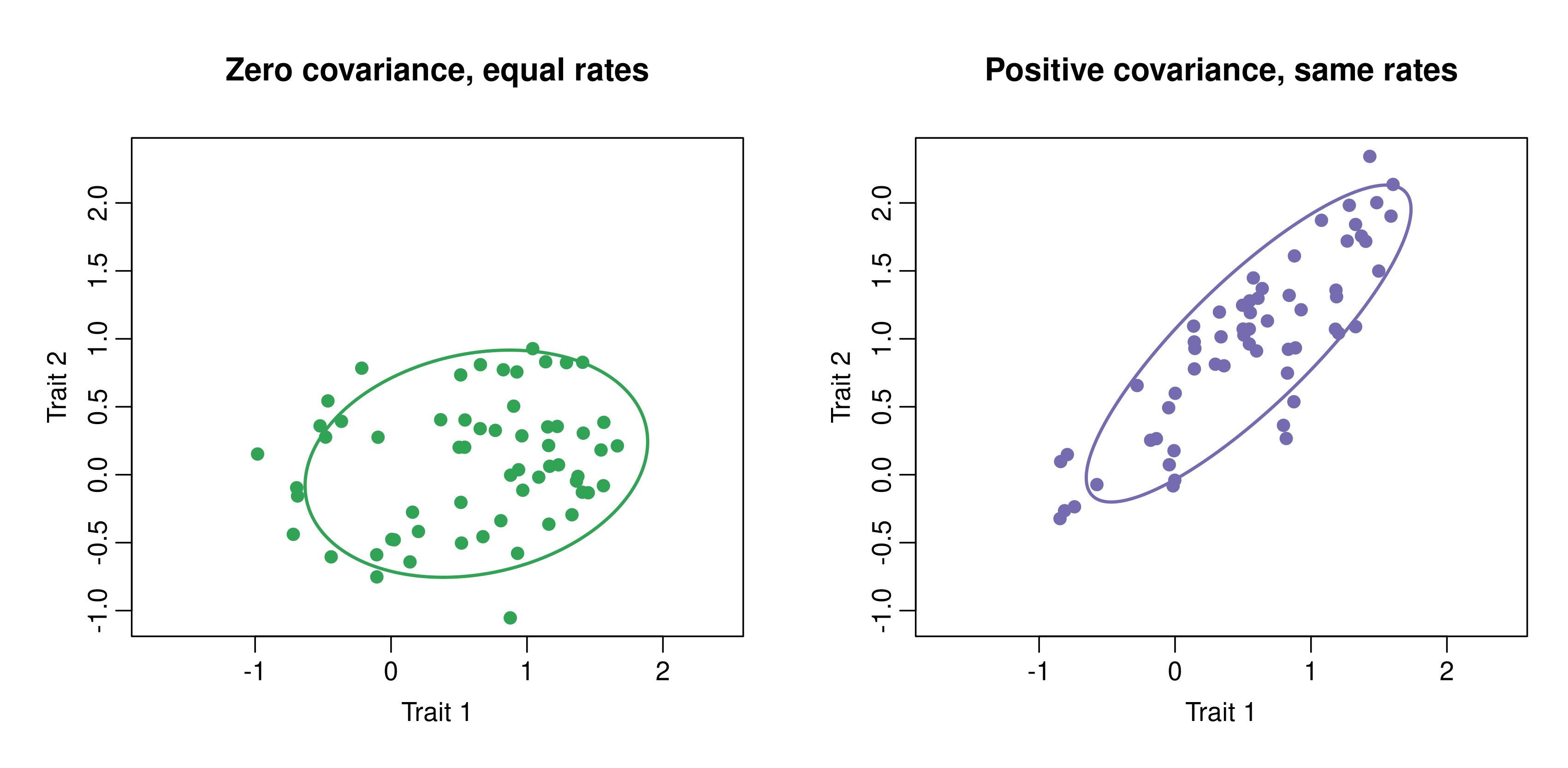
Figure 3. Two multivariate BM simulations on the same tree with matched trait-specific rates. The left matrix has zero covariance, whereas the right matrix has strong positive covariance. Because the diagonals are held constant across panels, the main visual change is in orientation and elongation rather than in overall rate. Ellipses summarize the sample covariance.

Figure 3 isolates covariance structure: both panels use the same diagonal rates, so the difference comes from the off-diagonal term rather than from faster or slower diffusion overall.

The matrices used in Figure 3 are:

sigma_zero_cov
#>      [,1] [,2]
#> [1,] 0.65 0.00
#> [2,] 0.00 0.65
sigma_pos_cov
#>      [,1] [,2]
#> [1,] 0.65 0.52
#> [2,] 0.52 0.65
round(cov2cor(sigma_pos_cov), 2)
#>      [,1] [,2]
#> [1,]  1.0  0.8
#> [2,]  0.8  1.0

Proportional rate shifts

A pure rate shift looks different. If $\mathbf{\Sigma}_2 = c \mathbf{\Sigma}_1$ for some positive constant $c$, the matrices are proportional in the Flury sense: they keep the same eigenvectors and the same relative eigenvalues, but one accumulates variance faster on every axis (Phillips and Arnold 1999).

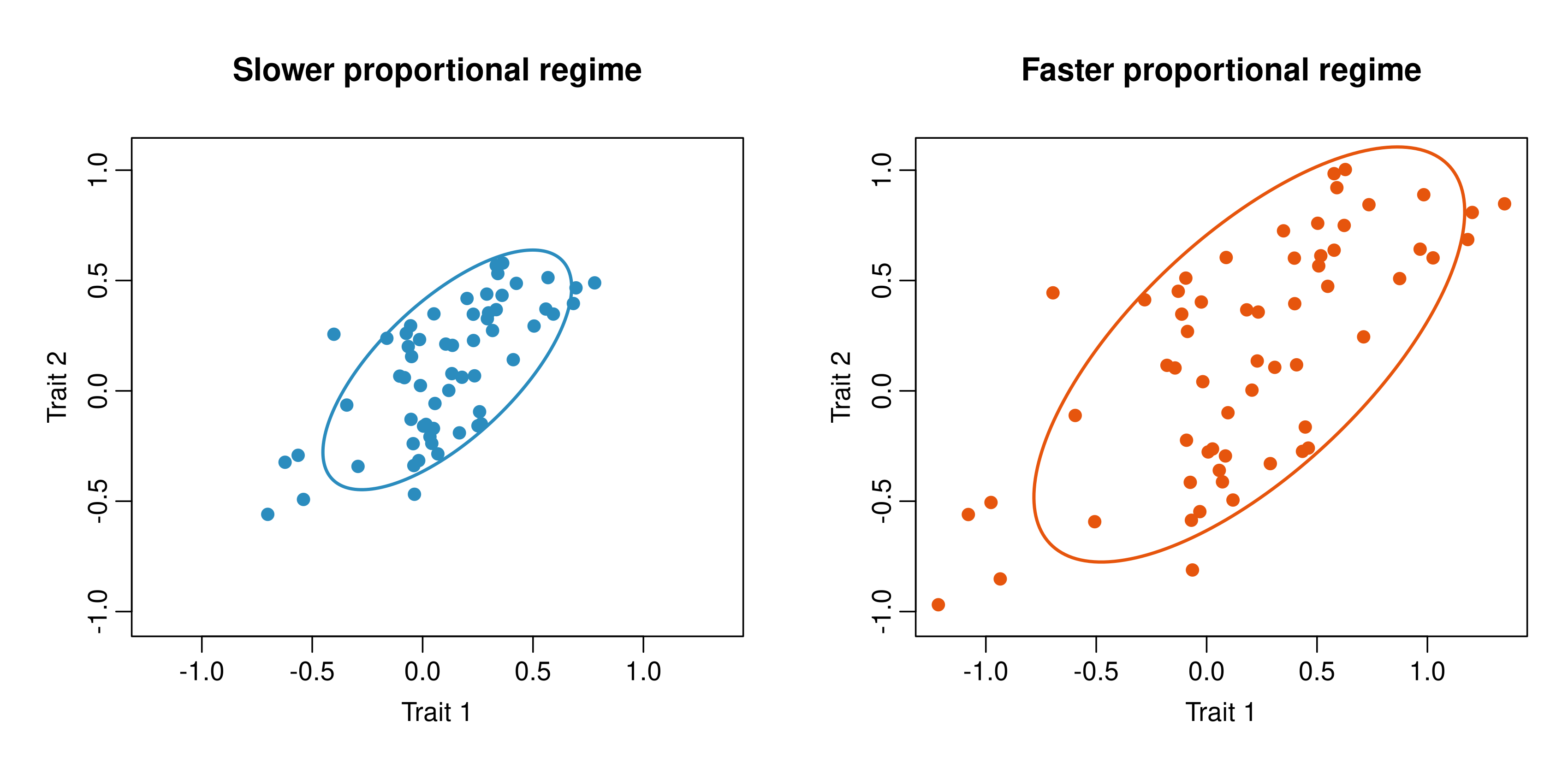
Figure 4. A proportional rate shift. The right matrix is a scalar multiple of the left, so the ellipses keep the same orientation and relative shape while expanding in size. Here the right panel is shown as an exact proportional expansion of the same realization, making the faster-versus-slower relationship visually explicit.

That distinction also shows up in empirical work. Stepanova et al. (2025) used this Flury-inspired ladder explicitly when comparing scincid lizard clades, distinguishing single-matrix, proportional rate-shift, shared-eigenvector, and fully different-eigenvector models. The broader point here is that a multivariate regime shift need not mean the same thing in every case: sometimes it is mostly about tempo, and sometimes it reflects a deeper reorganization of trait covariation.

In Figure 4, $\mathbf{\Sigma}_{\text{fast}} = 3 \mathbf{\Sigma}_{\text{slow}}$, so the faster regime is literally a proportional expansion of the slower one; the right panel is plotted as $\sqrt{3}$ times the same simulated realization.

Dimensionality and eigenvalues

It also helps to move from two traits to three. In three dimensions, covariance no longer just makes a cloud look round or elongated in a plane. It can make the cloud fill a volume, collapse toward a sheet, or narrow toward a ridge. In Figure 5, the three matrices all have the same trace, so the comparison is about how total variance is distributed across eigenvalues rather than about one regime simply having more variance overall.

Figure 5A.

Ball-Like Cloud

eigenvalues: 0.45, 0.45, 0.45

Figure 5B.

Sheet-Like Cloud

eigenvalues: 0.65, 0.65, 0.05

Figure 5C.

Ridge-Like Cloud

eigenvalues: 1.10, 0.15, 0.10

Figure 5. A three-trait comparison shown as three side-by-side 3D views. All three matrices have the same total variance (trace = 1.35), but they distribute that variance differently across axes. The green cloud is ball-like because it has three similar eigenvalues; the blue cloud is sheet-like because two eigenvalues dominate and one is small; the orange cloud is ridge-like because most variance sits on one axis. Each panel pairs centered simulated species values with the matching theoretical ellipsoid implied by that panel's generating covariance matrix.

The 3D example makes the same point from another angle. With comparable total variance, evolution can still look effectively three-dimensional, nearly planar, or almost one-dimensional. A simple rule of thumb is that the number of comparatively large eigenvalues tells you how many dimensions the cloud really fills.

From trait covariance to phylogenetic covariance

On a phylogeny, the full expected covariance has two ingredients: covariance among species and covariance among traits. A compact way to write it is $\mathbf{C} \otimes \mathbf{\Sigma}$, where $\mathbf{C}$ is the phylogenetic covariance matrix and $\otimes$ is the Kronecker product.

One intuitive way to read that expression is one species pair at a time. For any pair of species $i$ and $j$, the corresponding trait-covariance block is just $C_{ij}\mathbf{\Sigma}$. The main point is easy to lose in the notation: $\mathbf{C}$ does not introduce a new trait-covariance pattern for every species pair. It simply rescales the same template according to how much history that pair shares. In Figure 6, $C_{AB}$ stands in for one chosen entry from $\mathbf{C}$. In the HTML version, the slider lets you change that scalar directly. As it moves, the A-B block grows or shrinks, but the pattern set by $\mathbf{\Sigma}$ stays the same.

What does the phylogeny contribute?

Shared ancestry changes strength, not pattern

The slider changes only the shared-ancestry multiplier. The left panel stays fixed, while the right panel shows how strongly that same trait pattern appears between species A and B.

Shared history for A-B (CAB)

01

Current value: CAB = 0.60

Here the slider stands in for one entry of C. Moving it changes the strength of covariance, not the trait pattern itself.

Trait pattern stays fixed

Σ: trait-covariance template

Diagonal entries set relative variances; off-diagonal entries set covariance.

	Trait 1	Trait 2
Trait 1	0.90	0.50
Trait 2	0.50	0.70

This panel defines the pattern: tilt and aspect ratio come from Σ.

Use shared ancestry

CAB × Σ

→

Shared ancestry sets strength

A-B block in C ⊗ Σ

0.60× Σ

	Trait 1	Trait 2
Trait 1	0.54	0.30
Trait 2	0.30	0.42

At 0.60, every entry is 60% of the template, so the pattern is the same but weaker.

template Σscaled block

Figure 6. Shared ancestry changes strength, not pattern. Drag the shared-history value for one species pair. The left panel is the fixed trait-covariance template Σ; the right panel is the corresponding A-B block in C ⊗ Σ. As CAB changes, every entry in that block grows or shrinks together, so the ellipse changes size but not orientation.

The full matrix becomes easier to read if you think about it one species pair at a time. The same trait-covariance template is reused across every pair; what changes from block to block is only the scalar weight supplied by $\mathbf{C}$. Put differently, $\mathbf{C}$ controls how strong the covariance is between species, whereas $\mathbf{\Sigma}$ controls the pattern of covariance across traits. That is the statistical backbone of multivariate phylogenetic GLS and of the mvMORPH::mvgls fits used inside bifrost.

4. What Does a Branch-Specific Shift Mean?

A single-regime BM model assumes that the same covariance structure applies everywhere on the tree. bifrost is built for cases where that assumption may be too simple, and the practical question becomes whether some clade appears to evolve under a different multivariate rate structure from the background.

As the examples above suggest, that difference can take several forms. In the Flury hierarchy, which compares covariance matrices by how much eigenstructure they share, one regime might differ mainly by proportional scaling, another might retain the same major axes while changing variance along them, and a more dramatic shift can alter both size and orientation (Phillips and Arnold 1999). Even when the fitted comparison is phrased as BM versus BMM rather than as an explicit Flury test, that vocabulary is still useful for interpretation.

A shift is not just a change in where traits sit. It is a change in the geometry of the evolving trait cloud. Here we show the more dramatic end of that spectrum, where a descendant regime changes both size and orientation. The current bifrost search is narrower: it tests the proportional-scaling case, where descendant regimes differ in overall rate while retaining the same covariance geometry.

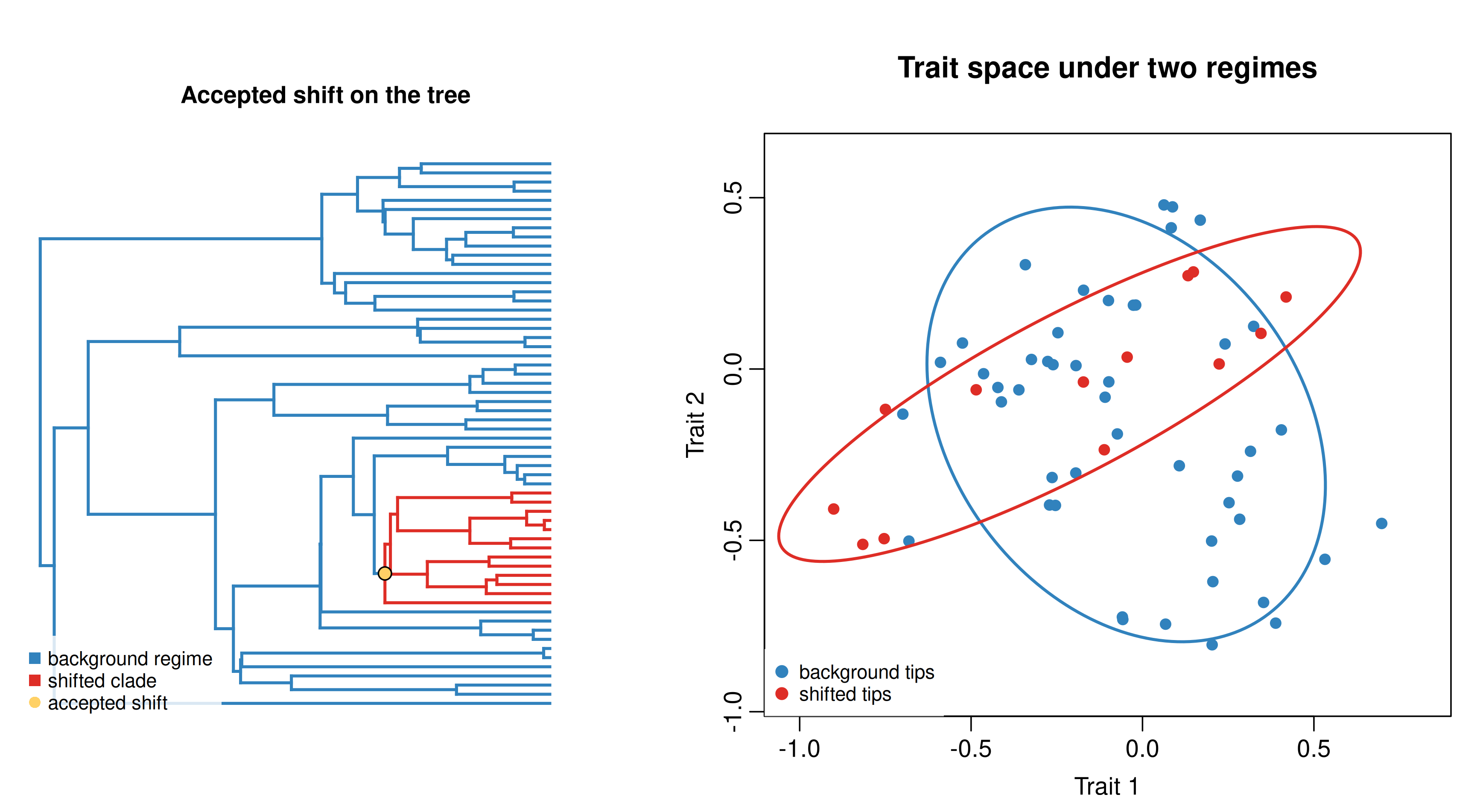
Figure 7. A two-regime BMM simulation. Left: one clade is painted with a derived regime on the tree. Right: the same simulation in trait space; the shifted clade (red) has a larger, differently oriented covariance ellipse than the background regime (blue). This is more than a simple proportional rate shift.

That example is conceptually useful, but it is not the literal target of searchOptimalConfiguration(). The search starts from a single-regime baseline, proposes internal nodes as candidate shifts, and asks whether allowing a descendant clade to occupy its own proportionally faster or slower multivariate regime gives a better approximation than the single-regime model, with enough improvement in fit to justify the added complexity.

For high-dimensional data, those comparisons are carried out with penalized-likelihood multivariate GLS machinery following the framework of Clavel, Aristide, and Morlon (2019). In the returned bifrost_search object, shift_nodes_no_uncertainty stores the accepted shift locations, VCVs stores the regime-specific variance-covariance matrices under the fitted proportional-scaling model, and baseline_ic, optimal_ic, and ic_weights summarize support for those extra regimes.

5. A Quantitative-Genetic Bridge

Readers coming from quantitative genetics will recognize the same geometry in the additive genetic variance-covariance matrix, $\mathbf{G}$. That resemblance is real. Both $\mathbf{G}$ and the macroevolutionary rate matrix are covariance matrices, so the same language of eigenvalues, eigenvectors, major axes, proportionality, and lines of least resistance naturally carries across scales (Lande 1979; Schluter 1996; Steppan, Phillips, and Houle 2002).

But the two matrices are not the same object. $\mathbf{G}$ describes additive genetic covariance within populations. By contrast, $\mathbf{\Sigma}$ or $\mathbf{R}$ in a phylogenetic BM model describes the rate at which trait variance accumulates among lineages. Under a narrow drift-only null, with a stable $\mathbf{G}$, constant effective population size, and branch lengths measured in generations, the expected evolutionary rate matrix is proportional to $\mathbf{G}/N_e$ (Lande 1979; Hohenlohe and Arnold 2008; Revell and Harmon 2008). Outside that special case, the macroevolutionary rate matrix can also reflect changing selection, moving optima, mutation, and evolution of $\mathbf{G}$ itself, so it should not be read as a direct estimate of the within-population $\mathbf{G}$-matrix.

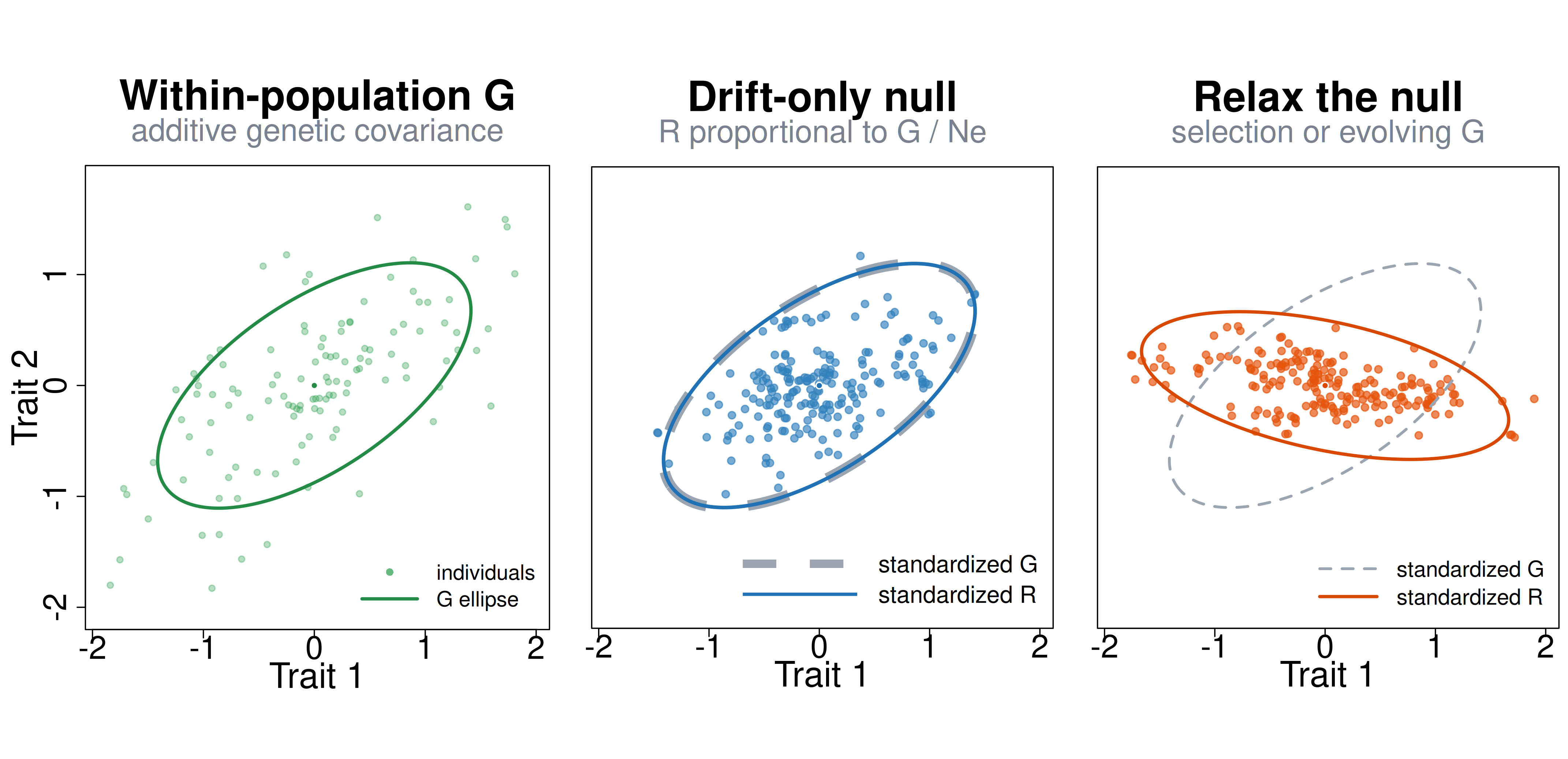
Figure 8. A schematic micro-to-macro bridge. Left: within-population additive genetic covariance, $\mathbf{G}$, shown as a cloud of individuals and its ellipse. The macro panels are rescaled to comparable size, so the comparison is about covariance geometry rather than raw units. Middle: under a narrow drift-only null, the macroevolutionary rate matrix is proportional to $\mathbf{G}/N_e$, so after standardization the dashed gray $\mathbf{G}$ ellipse and the blue $\mathbf{R}$ ellipse coincide. Right: once that null is relaxed, the among-lineage rate matrix can rotate or change shape relative to $\mathbf{G}$. Dashed gray ellipses show the standardized $\mathbf{G}$ geometry for comparison in the macro panels.

Practical Takeaways

• Brownian motion is useful because, on a phylogeny, it turns shared evolutionary history into an expected covariance structure among species.
• In multivariate data, the covariance matrix is part of the biological signal, not just a nuisance parameter.
• Regime differences can reflect overall rate scaling, changes in covariance geometry, or both.
• A branch-specific shift means that some clade is better described by a different multivariate rate structure than the background; in current bifrost, the search targets the proportional-scaling case.
• Under a narrow drift-only null, macroevolutionary rate geometry can be proportional to $\mathbf{G}/N_e$, but the phylogenetic rate matrix should not be read as the within-population $\mathbf{G}$-matrix itself.
• High-dimensional datasets require regularization and conservative model comparison, which is why bifrost relies on penalized-likelihood mvgls machinery.

Next Steps

If you want to keep going from here:

• Part 2, Whole-Tree Models, PCA, and bifrost, takes up whole-tree model limits, PCA-related cautions, and model-selection artifacts;
• the jaw-shape vignette shows an intercept-only morphometric workflow on Paleozoic fishes.

References

• Clavel, J., Aristide, L., and Morlon, H. (2019). A Penalized Likelihood Framework for High-Dimensional Phylogenetic Comparative Methods and an Application to New-World Monkeys Brain Evolution. https://doi.org/10.1093/sysbio/syy045
• Felsenstein, J. (1985). Phylogenies and the Comparative Method. https://doi.org/10.1086/284325
• Hohenlohe, P. A., and Arnold, S. J. (2008). MIPoD: A Hypothesis-Test Framework for Microevolutionary Inference From Patterns of Divergence. https://doi.org/10.1086/527498
• Lande, R. (1979). Quantitative Genetic Analysis of Multivariate Evolution, Applied to Brain:Body Size Allometry. https://doi.org/10.1111/j.1558-5646.1979.tb04694.x
• Phillips, P. C., and Arnold, S. J. (1999). Hierarchical Comparison of Genetic Variance-Covariance Matrices. I. Using the Flury Hierarchy. https://doi.org/10.1111/j.1558-5646.1999.tb05414.x
• Revell, L. J., and Harmon, L. J. (2008). Testing Quantitative Genetic Hypotheses About the Evolutionary Rate Matrix for Continuous Characters. https://lukejharmon.github.io/assets/Revell_and_Harmon_2008.pdf
• Schluter, D. (1996). Adaptive Radiation Along Genetic Lines of Least Resistance. https://doi.org/10.1111/j.1558-5646.1996.tb03563.x
• Steppan, S. J., Phillips, P. C., and Houle, D. (2002). Comparative Quantitative Genetics: Evolution of the G Matrix. https://www.bio.fsu.edu/dhoule/Publications/steppanetal2002.pdf
• Stepanova, N., Boyko, J. D., Lin, J., Davis Rabosky, A. R., and Rabosky, D. L. (2025). Punctuated Versus Gradual Shifts in the Multivariate Evolutionary Process: A Test With Paired Radiations of Scincid Lizards. https://doi.org/10.1093/sysbio/syaf002

Software Used in This Vignette

• Clavel, J., Escarguel, G., and Merceron, G. (2015). mvMORPH: an R package for fitting multivariate evolutionary models to morphometric data. Methods in Ecology and Evolution, 6(11), 1311-1319. https://doi.org/10.1111/2041-210X.12420
• Ligges, U., and Mächler, M. (2003). Scatterplot3d - an R Package for Visualizing Multivariate Data. Journal of Statistical Software, 8(11), 1-20. https://doi.org/10.18637/jss.v008.i11
• Paradis, E., and Schliep, K. (2019). ape 5.0: an environment for modern phylogenetics and evolutionary analyses in R. Bioinformatics, 35, 526-528. https://doi.org/10.1093/bioinformatics/bty633
• Revell, L. J. (2024). phytools 2.0: an updated R ecosystem for phylogenetic comparative methods (and other things). PeerJ, 12, e16505. https://doi.org/10.7717/peerj.16505
• Sievert, C. (2020). Interactive Web-Based Data Visualization with R, plotly, and shiny. Chapman and Hall/CRC. https://plotly-r.com
• Cheng, J., Sievert, C., Schloerke, B., Chang, W., Xie, Y., and Allen, J. (2024). htmltools: Tools for HTML. R package version 0.5.8.1. https://CRAN.R-project.org/package=htmltools

AI Assistance

This vignette was developed with assistance from OpenAI tools for drafting, editing, and figure refinement; all scientific content, interpretation, and final decisions were reviewed by the authors.