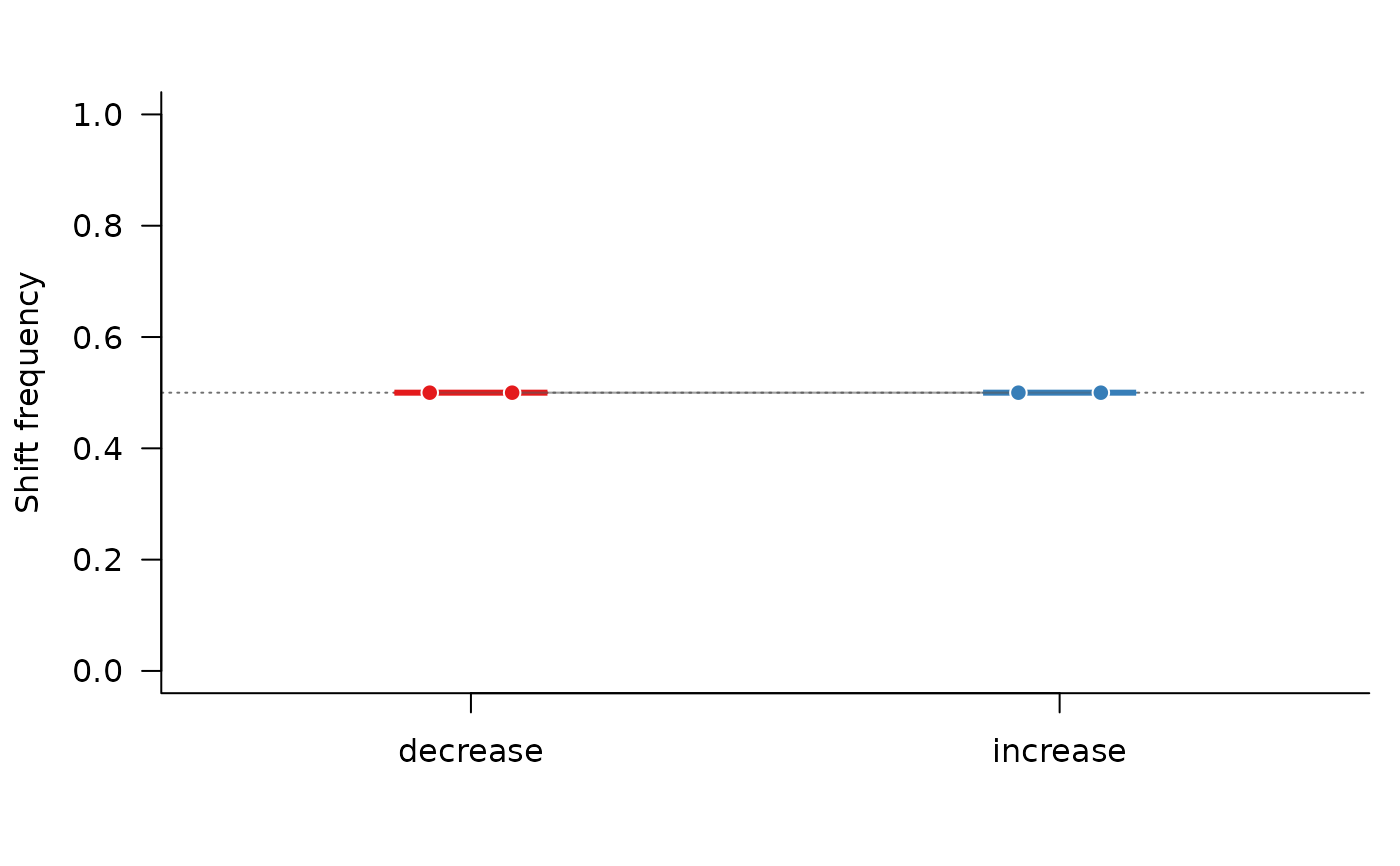
Plot One Shift Count Or Frequency Comparison — plot.shift_magnitude

Summarize inferred rate increases and decreases for one set of search outputs. The default paired frequency plot mirrors the count/frequency comparison used for Berv et al. (2026) Supplementary Figure 5.

Usage

# S3 method for class 'shift_magnitude_counts'
plot(
  x,
  statistic = c("frequency", "count"),
  colors = c(increase = "#377eb8", decrease = "#e41a1c"),
  point_cex = 1.15,
  line_col = grDevices::adjustcolor("grey35", alpha.f = 0.35),
  boxplot = TRUE,
  paired_lines = TRUE,
  paired_test = TRUE,
  reference_line = NULL,
  ylim = NULL,
  ylab = NULL,
  main = NULL,
  mar = c(4.5, 4.2, 2.4, 0.8),
  oma = c(0, 0, 0, 0),
  ...
)

Arguments

x: A shift_magnitude_counts object.
statistic: Plot "frequency" or raw "count" values.
colors: Named colors for "increase" and "decrease".
point_cex: Point size for run-level observations.
line_col: Color for paired run-level segments.
boxplot: Logical; overlay compact boxplots.
paired_lines: Logical; draw paired decrease-to-increase segments for each run.
paired_test: Logical; annotate the plot with a paired Wilcoxon test when at least two runs are available.
reference_line: Optional horizontal reference line. Defaults to 0.5 for frequencies and no line for counts.
ylim: Optional common y-axis limits.
ylab, main: Plot labels.
mar, oma: Graphical margins passed to graphics::par().
...: Additional graphical parameters passed to graphics::plot().

Value

Invisibly returns a list with the count data, paired tests, and plot settings.

Examples

transitions <- data.frame(
  rate_change = c("root", "increase", "increase", "decrease", "decrease"),
  rate_delta = c(NA, 3, 4, -1, -2)
)
counts <- shift_magnitude_counts(list(run1 = transitions, run2 = transitions))
plot(counts)